
L.T. Lee
Department of Computer Science and Engineering, Tatung University, Taipei 10452, Taiwan
C.W. Chen
Department of Computer Science and Engineering, Tatung University, Taipei 10452, Taiwan
Information Technology Journal
Year: 2008 | Volume: 7 | Issue: 5 | Page No.: 737-745


ABSTRACT
Sensing and detecting of the events through sensor networks is one of popular research areas. Sensors can help us not only to detect the pollution, but also to monitor the environment that is beyond our reach. When sensor nodes go on their missions, synchronization is a very important issue. If the clock in the all sensors is not synchronized, as they detect the event and send the data to the sink in the sensor network, the sequence of data with time stamp will be disorder. It is harder to read and identify data. Prior to our research, there are a lot of methods to synchronize all nodes in the sensor network, for example, Lightweight time synchronization for sensor networks (LTS), centralized multi-hop lightweight tree-based synchronization (CLTS), pulse-coupled, cluster-header and so on. The methods between the pulse-coupled and cluster-header have the same characters. When the sensor networks are synchronizing, the nodes in the pulse-coupled way and the cluster-header method will provide their own information to sync each other. In present study, we will compare the different between the pulse-coupled method and the cluster-header method.
PDF Abstract XML References Citation
How to cite this article
L.T. Lee and C.W. Chen, 2008. Synchronizing Sensor Networks with Pulse Coupled and Cluster Based Approaches. Information Technology Journal, 7: 737-745.
DOI: 10.3923/itj.2008.737.745
URL: https://scialert.net/abstract/?doi=itj.2008.737.745
DOI: 10.3923/itj.2008.737.745
URL: https://scialert.net/abstract/?doi=itj.2008.737.745
INTRODUCTION
Nowadays, a sensor network can be applied to more and more areas. Some of the examples are listed below. People can use sensors to detect air pollution. The firemen can observe that the building is on fire and decide the best time to rescue the victims in the fire. The car installed with many sensors can help us to monitor the traffic situation (Arampatzis et al., 2005). There are many ways we can apply the technology of sensor networks.
In the earlier examples, the sensor nodes are placed in a fixed place. The researchers will use hundreds of thousands of sensor for the mission which they are interested in. Let’s focus on the whole sensor network. There are four parts in the sensor network, i.e., the sensor nodes, the sink, the user computers and the internet. The sensor network which has many nodes has own algorithms to communicate with each other to detect an object or an event. The missions of the sink are to collect data, synchronize and control the sensors in the sensor network among other important tasks. As a sink collects data, we need a communication channel to send data to the user computers. The internet can provide a link services to communicate between users and the sensor network. The internet media includes Ethernets, satellites, 3G, WiMAX and so on. The data from the sink can be processed and analyzed by the user computers. The results can be shown in the user computers. The sensor network’s architecture is shown in Fig. 1.
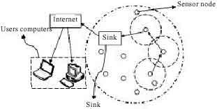 | |
| Fig. 1: | Sensor networks architecture |
A sensor includes the sensing unit, the processing unit, the communication unit and the power unit. The job of the sensing unit is detecting objects, people, events and so on. The power unit is another important component. If the power unit can store more energy, the sensor may last longer. The processing unit just collects and analyzes the data from the nodes. A transceiver and a mobile device are two parts of the communication unit. The communication unit delivers the packets between nodes and the sink. Figure 2 demonstrates these components in (Akyildiz et al., 2002). They can communicate with each other. On the other hand, the power consumption is a problem in the sensor network. The sensor nodes are small and cheap. If the sensor nodes equip a big battery, the cost will be raised. In generally, the battery in the sensor nodes is small. Hence, the sensor may not last longer. Some researchers proposed mechanisms that put idle sensor nodes to the sleep mode in the hope of reducing power consumption. When the sensor nodes wake up, they will synchronize to adjust the clocks in the sensor nodes. That is why the sensor network needs to synchronize each other.
 | |
| Fig. 2: | The components of a typical sensor node |
Synchronization mainly helps the clock of the sensor to be consistent with those of other sensors. In those synchronization methods, we choose the pulse-coupled synchronization, because the pulse-coupled method is the biology synchronization. It is a good research topic. The idea of pulse-coupled is from fireflies (Mirollo and Strogatz, 1990.). When the sunset comes, fireflies will gather on trees together. Initially, they flash rather independently. However, after a while the flash will be synchronous. There is an interesting how to learn from the fireflies’ synchronization.
Another way of synchronization is to use cluster-header. The members of cluster-header are header, gateway and sensor nodes. The character of cluster-header synchronization is that one sensor network is cut to many groups and each group has a header. The header of the group receives the data from the sensor nodes in the same group and from the gateways shared with other headers. Gateways may exist in a group since the group can share nodes with other neighboring groups.
RELATIVE WORK
Here, we study about Time-diffusion synchronization protocol and Time-sync protocol.
Time-diffusion synchronization protocol: Akyildiz and Su (2006) proposed a time-diffusion synchronization protocol (TDP) for wireless sensor networks (Su and Akyildiz, 2005.). In TDP, it has four procedures including Peer Evaluation Procedure (PEP), time diffusion procedure (TP), election (reelection) of master (diffused) leader node procedure (ERP) and Time Adjustment Algorithm (TAA).
TDP divides time into active and inactive periods as shown in Fig. 3. In the active period of τ sec, the master nodes are elected and time synchronization is carried out. The active period is further divided into even smaller intervals of δ sec. The initial multiple trees-like structures need to be created before sending time information messages. There are many master nodes selected as possible candidates of roots in the trees. The selection of master nodes is basically random. However, a muster node needs to meet some requirements in its clock and power level. These trees are used as the platform for time distribution. The level indexes of the tree are assigned to the nodes according to their positions in the structure. For example, the root node is at level 0 while its children and descendant are at level 1 and beyond. The master nodes or the associated diffused leader nodes communicate with their immediate children diffused leader nodes for time synchronization.
 | |
| Fig. 3: | TDP active/inactive schedule |
 | |
| Fig. 4: | Handshake of timing information message |
The root nodes repeat the time diffusion procedure (TP) in each of the periods. In the TP, the master nodes diffuse timing information messages at every δ second for duration of τ sec. The message contains the round trip time, master node’s ID, weight value, etc. Then, the handshake is carried out and repeated between a master node and its associated diffused leader nodes or between a diffused leader and its children diffused leaders as Fig. 4 shows. The TP uses the built trees to synchronize the network.
The Election/Reelection Procedure (ERP) is based on a random function biased to favor nodes with more power reservation. It balances the workload for all nodes in the network. And, the procedure includes two algorithms, the False Ticker Isolation Algorithm (FIA) and the Load Distribution Algorithm (LDA). The FIA has a threshold to exclude nodes with drastically different local clocks from being the master nodes. The threshold is compared against the Allan variance in the PEP. If it is greater than the threshold, the node will be filtered out. The LDA is capable of balancing out the energy consumption among the nodes. It uses the value, λ, reflecting the ratio of current energy level, to determine if a node should be considered as a master node. If the node’s λ value is greater than a threshold, then it is more likely to be reelected as a master node or a diffusion leader. In the time adjustment procedure (TAA), a sensor node adjusts its local clock based on the difference between the clock and that of the master node or the diffused leader node. In addition, a weight is calculated to be used as a correction ratio. The calculation considers the number of hops from the master node or the diffused leader node to the local node. The multiplication of the weight and the time difference results in the amount of adjustment that should be made to the local clock.
The TDP architecture including ERP, PEP and TP is shown in Fig. 5. First, the initialize pulse indicates the assignment of master nodes sent out by the sink. Then, the master nodes exchange messages with their neighbor nodes. It repeats the ERP to determine the diffused leader nodes and form tree-like structures. However, the FIA is not invoked in the initial round. Starting from the second round, the FIA and the LDA are repeated every τ sec to identify qualified master nodes. The τ value can be optimized for various sizes of wireless sensor networks. In general, it is linear to the maximum number of layers in the created trees.
The pros and cons of this protocol are discussed in the following. The protocol applies many supporting algorithms to curtail energy consumption and achieve time synchronization. It allows the nodes to reach a synchronous time with small errors. It is adaptive for both static and mobile sensor network environments due to the periodic construction of the multiple tree-like structures.
 | |
| Fig. 5: | TDP architecture |
The protocol considers numerous realistic aspects and contains a couple of supporting procedures. They inevitably incur more message and computation complexity when compared with other less thorough mechanisms. For example, its peer evaluation procedure requires intensive message exchanges to remove false nodes. Since the cost of building the multiple tree-like structures is not explicitly discussed in the paper, we speculate that it may be overwhelming if the sole purpose of the structures is synchronization. Furthermore, the performance comparison against other synchronization schemes is mostly missing in the paper. It is unclear if this complicated design is superior to other simpler schemes.
Timing-sync protocol: Ganeriwal et al. (2003) proposed a time synchronization protocol, which is called the Timing-sync Protocol for Sensor Networks (TPSN). It aims at providing network-wide time synchronization in the sensor network.
The TPSN works in two phases for time synchronization. In the initial phase called the Level Discovery Phase (LDP), a hierarchical tree structure is established in the network. Figure 6 shows the propagation of the level discovery phase. The second phase known as Synchronization Phase (SP) performs a pair-wise synchronization along the edges of the discovered tree. It establishes a global time throughout the network. Eventually, all nodes in the network synchronize their clocks to the reference node (known as the root node). The level discovery phase starts at the root node or the initiator (known as the sink). The root node is assigned as level number 0 and initiates this process by broadcasting a level discovery packet to its neighbor nodes. This packet contains the identity and the level number of its sender. When the neighbor nodes of the root node receive this packet, they will assign themselves a level number accordingly. The assigned level number is greater than the level contained in the packet they just received by one. This phase will continue until all nodes in this sensing field obtain their level numbers.
 | |
| Fig. 6: | LDP of TPSN |
 | |
| Fig. 7: | Two-way message exchange method |
Figure 7 shows the two-way message exchange between nodes A and B. T1 and T4 are the measured time epochs by the local clock of A. On the other hand, T2 and T3 are measured by the local clock of B. At the time T1, node A sends a synchronization pulse packet to node B. This synchronization pulse packet contains two pieces of information, (i) the level number of A and (ii) the value of T1. At the time T2, node B receives the packet and records the receiving time locally. T2, of the clock of node B, is equal to T1+Δ+d, where Δ and d represent the clock drift time between the pair of nodes and the propagation delay, respectively. It should be noted that Δ may not be time invariant. However, it is considered constant for the short period of the two-way exchange process. At the time T3, node B finishes processing synchronization pulse packet and sends back an acknowledgment packet to node A. This acknowledgment packet contains the level number of B and the values of T1, T2 and T3. At the time T4, node A receives the packet. Similarly, T4, of the clock of node A, is equal to T3-Δ+d. Finally, these parameters are used by node A to calculate the Δ and d in the following equations:
(1) |
(2) |
where, the Δ and d are calculated by Eq. 1 and 2 accordingly, the node A can correct its clock so that it synchronizes to node B.
After the LDP, the synchronization phase will begin at the root node. Base on the established tree structure, the Synchronization Phase (SP) starts its process at the root node. It broadcasts a synchronization pulse packet to its neighbor nodes. Each neighbor node will use the two-way message exchange method to synchronize with the root node. After synchronizing with the root node, its neighbor nodes will continue to broadcast their synchronization pulse packets to synchronize with their respective neighbor nodes. Eventually all nodes in the sensing field are synchronized to the root node.
The pros and cons of this protocol are discussed in the following. The protocol can reach time synchronization by the two-way message exchange method. And, there is no complicated step to create the tree-like structure. But, it still divides into two steps to complete time synchronization. In a stretched network, the protocol will need to spend much time to create the tree-like structure because it will have a greater number of levels. As a result, the synchronization convergence time increases linearly as the number of levels grows since synchronization is achieved one level at a time. In summary, this type of protocols suffers from the tree construction cost and poor scalability in convergence time.
PULSE COUPLED AND CLUSTER HEADER SYNCHRONIZATION
Pulse-coupled synchronization: The pulse is one of interesting phenomenons in Natural. The famous pulse example is the heart-beat, the fireflies and so on. The property with the pulse-coupled is used to the pulse to sync each other. In South Asia, the fireflies flock together under trees and flash synchronizingly in the evening (Tyrrell et al., 2006; Mirollo and Strogatz, 1990). Initial, the flash with light fireflies is disorder. For a long time, the light of fireflies will be synchronization. Mirollo and Strogatz (1990) proposed the mathematics about the pulse-coupled in 1990. After the mathematics (Barbarossa and Celano, 2005), applied the mathematics in the synchronization of wireless sensor network. This mathematics model for sensor network is one of important synchronization way. The architecture of pulse-coupled sensor network is a fully-mesh sensor network, the sensor nodes will connection and sync each other, the network don’t need any cluster header, every node is a header to emit singles to other nodes.
The mathematical model of oscillators is as (x), each oscillator i, 1≤i≤N, The state is described by a variable xi, it is similar to a voltage-like variable in a RC-circuit and its evolution and interactions are described by a set of differential equations (Tyrrell et al., 2006):
(3) |
where, k0 controls the uncoupled oscillators and Sij is the coupling strength between oscillators. When xi = xth, where xth is the state variable threshold, one oscillator will say fire, at the same time, its state is reset to 0 and it emits a pulse out, the pulse can change the state of other oscillators. The function of oscillator coupling is defined as:
(4) |
where, ![]() represents the mth firing time of oscillator j and δ(t) is dirac delta function. The dirac delta function is a limit scope function.
represents the mth firing time of oscillator j and δ(t) is dirac delta function. The dirac delta function is a limit scope function.
Figure 9 shows the state of oscillators. In the Fig. 9A, it plots the time evolution of the phase function during one period, at T period the oscillator emits its single. In the Fig. 9B, it plots the time evolution of the phase function when receiving the pulse. Renato and Strogatz (1990) proposed the formula which adjusts the phase of sensor nodes as follows:
(5) |
Barbarossa and Celano (2005) proposed a new protocol with information propagation based on mutual coupling of dynamic systems. The information spreads as the result of the couplings among adjacent nodes. One example is that the coupled nodes mutually act to adapt their clocks. In the protocol, we can reach time synchronization by using the mathematical equation:
(6) |
where, θi(t) is the state function of the ith sensor; aij are real variables that describe the coupling between sensors i and j; k is a control loop gain; ci is a coefficient that quantifies the attitude of the i-th sensor to adapt its values; wi is an initial condition given by the initial pulsation. For the function, F(.), we must use an monotonically increasing nonlinear odd function. The possible choices for F(x) are:
(7) |
or
(8) |
In this coupled dynamic system, a malicious node may prevent the entire network from synchronization by refusing to follow the algorithm. It is important to know the synchronization convergent time. If it takes too long or if there are too many message exchanges involved, then this approach is not justified. Through local coupling, we can gather all the information present in each node without any sensor fusion center. The mutually coupled dynamic system performs as a globally optimal fusion center. Each coupled system can be of any size or contain any number of sensors. For example, each node is coupled with four other nodes. If the sensor network has 20 nodes, it has 4 couples. Then it must send the result to the base station. It consumes more energy than the protocol with fusion centers.
 | |
| Fig. 8: | The phase of pulse-coupled with the wireless applications |
 | |
| Fig. 9: | Time evolution of the phase function |
There are many papers about the applications of pulse-coupled synchronization. Tyrrell et al. (2006) discussed that the pulse-coupled synchronization is applied to real wireless network. The propagation delay in the pulse-coupled theory doesn’t be considered. But the distance of propagation in ad hoc wireless network is limited by buildings, walls and so on. For this problem, the authors proposed a method to solve the propagation delay. They suppose when a node reach a level to fire, the node don’t receive any singles from its neighbors. It can help the whole wireless network be stable. The structure of stable is as Fig. 8:
 | |
| Fig. 10: | Initialization in the passive clustering method |
 | |
| Fig. 11: | The structure of cluster-header sensor network |
Cluster-header synchronization: Cluster-header is one of synchronization methods in the sensor network field (Kwon et al., 2003). Mamun-Or-Rashid et al. (2005) proposed a protocol called passive cluster based clock synchronization in sensor networks . It is a two-hop way to synchronize. The distance between the header and node in the sensor network isn’t over 3-hops. In the cluster-header sensor network, there are three components: (1) cluster header, (2) gateway and (3) ordinary node. The structure of cluster-header sensor network is Fig. 11 and 12. When the synchronization starts, the nodes are received the information from the cluster passively. It calls passive clustering.
As the network synchronizes in the passive clustering, there are four statuses for clustering header: (a) Initial, (b) Cluster header, (c) Gateway and (d) Ordinary. Every node becomes cluster header possible. The nodes in the sensor network will be chosen as temp header as Fig. 10a. They can determine sensing range and send initial messages to the nodes which in the sensing range. If the nodes in the sensing range receive the message from temp header, the initial nodes can be the candidate for cluster header as Fig. 10b. The node will be selected a cluster header by first declaration wins. At this time, the cluster header will remember its group of sensor nodes as Fig. 10c. The normal nodes call ordinary nodes. If the position of nodes covers two or three groups, the nodes become gateway. The mission of gateway is reposing to deliver the different information to the other cluster header. The cluster header accounts the average faster from the gateways. The synchronization algorithm is as Table 1.
 | |
| Fig. 12: | The synchronization of cluster-header sensor network |
| Table 1: | The algorithm of cluster-header |
 | |
SIMULATION
To understand the detail of synchronization with the pulse-coupled method and the cluster-header method, we simulate the two methods. We setup the positions of the sensor nodes randomly as Fig. 13 and 14. The simulation parameter between the pulse-coupled method and the cluster-header method includes 500 nodes, 500 times of synchronization. At the same time, the algorithm in the pulse-coupled method is used as (6) and the F function which we choose is used as (7). The algorithm in the pulse-coupled method is as Table 1. Besides, we simulate the abnormal synchronization. We suppose that a mischievous node disturbs the whole sensor network. We set a mischievous node in both of the synchronization methods. The mischievous nodes can make two conditions of synchronization: one is that the clock of mischievous nodes is fixed. Another one is that the clock of mischievous nodes is up and down between normal clocks.
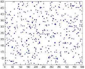 | |
| Fig. 13: | The position of the sensor nodes for cluster-header method |
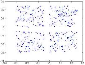 | |
| Fig. 14: | The position of the sensor nodes for pulse-coupled method |
The normal synchronization of the pulse-coupled method and the cluster-header method shows as Fig. 15 and 16. In the pulse-coupled method, the coverage time is very fast. It just costs 30 cycles to synchronize because of the nodes provide itself information to synchronize. Every node is header to sync each other easily. In the cluster-header method, the coverage time is slower than pulse-coupled method because the synchronization is sync by the header, gateways. The influence of cluster-header method isn’t better direct than the influence of pulse-coupled method.
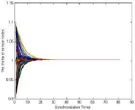 | |
| Fig. 15: | The result of synchronization in the pulse-coupled method |
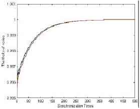 | |
| Fig. 16: | The result of synchronization in the cluster-header method |
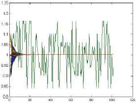
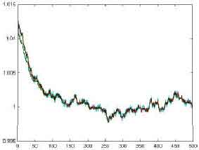
Figure 17 and 18 show the abnormal synchronization. When the sensor network is synchronizing, there is a mischievous node to affect the whole sensor network. In the Fig. 16, we can obtain the fault tolerant in the pulse-coupled method is higher because the mischievous node don’t’ effect other nodes directly. In the Fig. 17, the mischievous node affects the whole sensor network very worst. The header is the same group with the mischievous node. The header receives the information of mischievous node. It can make the average in that group higher or lower. At the same time, the average with higher or lower is sent to the gateway in the other groups and the gateways send the average with higher or lower to the header in the other groups. The result can make the whole sensor network unstable.
Another condition is one fixed information node. In our simulation, the clock of all nodes will be toward to the mischievous nodes between the pulse-coupled method and cluster-header method.
 | |
| Fig. 17: | The result of abnormal synchronization in the pulse-coupled method |
 | |
| Fig. 18: | The result of abnormal synchronization in the cluster-header method |
The fixed node doesn’t be affected by the other node, but the other nodes are affected by the fixed node. This condition for the sensor network isn’t a big problem; another one condition can make the sensor network unstable. We need pay attention for the mischievous node.
CONCLUSION AND FUTURE WORK
In our research, we focus on the two synchronization methods of pulse-coupled and cluster-header because the two methods of synchronization are too similar. There is a simulation in pulse-coupled and cluster-header. The parameter of simulation is 500 nodes, 250 sensing range, 500x500 area and 500 cycles in the synchronization. We can find the pulse-coupled needs 50,000,000 packets and the cluster-header needs 624,949,288 packets to sync all nodes. The example shows they need a lot of packets to sync each other. In the other research, the other synchronizations just need one node with clock information to send the other nodes. But, the pulse-coupled and cluster-header need all nodes with clock information to sync each other. It means every node in the pulse-coupled and cluster-header provides itself clock information to sync the other node. We also discuss the different characteristic between pulse-coupled and cluster-header. The pulse-coupled uses the characteristic of biology in synchronization. Every node will sync each other and the clock information node in far way will affect the other node one by one. The way of synchronization doesn’t affect the other nodes directly and fast, so fault tolerant is higher. The Pulse-coupled method doesn’t use any algorithms to cluster and the synchronization can be implemented immediately. It is the benefit for pulse-coupled, because it doesn’t waste the power in the sensor node. For sensor power consume in pulse-coupled, the nodes consume more power when the synchronization is running. In cluster-header, the clock information is delivered by gateways and headers and the influence is directly, so fault tolerant isn’t good. It is cluster by cluster algorithms to sync each other. In cluster-header, it uses the characteristic of group in synchronization. For sensor power consuming in cluster-header, the nodes consume less power when the synchronization is running.
| Table 2: | The Characteristic of pulse-coupled synchronization and cluster-header |
 | |
Comparing the two synchronization methods of pulse-coupled and cluster-header is an interesting topic. In this research, we find the same and the different between pulse-coupled and cluster-header as Table 2. At the same time, if there are some mischievous nodes in the sensor network, they don’t make the all sensor synchronization completely. It is an interesting problem which how to control the mischievous nodes. We will focus on the problem with the mischievous nodes, because a few papers talk about the mischievous nodes and they don’t propose the solving ways.
REFERENCES
- Tyrrell, A., G. Auer and C. Bettstetter, 2006. Fireflies as role models for synchronization in ad hoc network, 2006 Bio-inspried models of network. Inform. Comput. Syst.
CrossRef - Akyildiz, I.F., W. Su, Y. Sankarasubramaniam and E. Cayirci, 2002. A survey on sensor networks. IEEE Commun. Mag., 40: 102-114.
CrossRefDirect Link - Mamun-Or-Rashid, M., C.S. Hong and C.H. In, 2005. Passive cluster based clock synchronization in sensor network. Proceedings of the Advanced Industrial Conference on Telecommunications/Service Assurance with Partial and Intermittent Resources Conference/E-Learning on Telecommunications Workshop, July 17-20, 2005, Washington, DC. USA., pp: 340-345.
CrossRef - Mirollo, R.E. and S.H. Strogatz, 1990. Synchronization of pulse-coupled biological oscillators. SIAM J. Applied Math., 50: 1645-1662.
CrossRef - Barbarossa, S. and F. Celano, 2005. Self-organizing sensor networks designed as a population of mutually coupled oscillators. Proceedings of the 6th Workshop on Signal Processing Advances in Wireless Communications, June 5-8, 2005, Cannes, France, pp: 475-479.
CrossRef - Ganeriwal, S., R. Kumar and M.B. Srivastava, 2003. Timing-sync protocol for sensor networks. Proceedings of the 1st International Conference on Embedded Networked Sensor Systems, November 5-7, 2003, New York, USA., pp: 138-149.
CrossRef - Kwon, T.J., M. Gerla, V.K. Varma, M. Barton and T.R. Hsing, 2003. Efficient flooding with passive clustering-an overhead-free selective forward mechanism for ad hoc/sensor networks. Proc. IEEE, 91: 1210-1220.
CrossRef - Su, W. and I.F. Akyildiz, 2005. Time-diffusion synchronization protocol for wireless sensor networks. IEEE/ACM Trans. Network., 13: 384-397.
CrossRef