
Yang Hui
College of Science, Xi`an University of Science and Technology, Xi`an, China
Information Technology Journal
Year: 2011 | Volume: 10 | Issue: 5 | Page No.: 1038-1043


ABSTRACT
With regard to a wireless sensor network, organizing sensors into a hierarchy of clusters with an objective of minimizing the total spent energy to communicate the information gathered by sensors to the information-processing center, rough set theory can serve as a useful pre-processing tool, removing superfluous attributes and suggesting validated rules and models on an objective and global basis, i.e., without any tuning for this particular application. Actually, data management for the WSN is very complex and there is wide scope for further research on intelligent data collection and dynamic reduction in this area so as to make the schemas more applicable. This study discusse the distance learning algorithm DLA (distance learning algorithm) to achieve, as well as it’s the modern teaching of universal significance. Inductive learning is a research area in Artificial Intelligence. It has been used to mode1 the knowledge of human experts by using a carefully chosen sample of expert decisions to infer decision rules. Rough set based inductive learning uses rough set.
PDF Abstract XML References Citation
Received: November 29, 2010;
Accepted: February 14, 2011;
Published: March 18, 2011
How to cite this article
Yang Hui, 2011. Ad Hoc Networks Based on Rough Set Distance Leaming Method. Information Technology Journal, 10: 1038-1043.
DOI: 10.3923/itj.2011.1038.1043
URL: https://scialert.net/abstract/?doi=itj.2011.1038.1043
DOI: 10.3923/itj.2011.1038.1043
URL: https://scialert.net/abstract/?doi=itj.2011.1038.1043
INTRODUCTION
A symbolic approach to achieve this aim is the rough set theory which identifies partial or total dependencies (i.e., cause-effect relations) in databases, eliminates redundant data and gives approach to null values, missing data, dynamic data and others (Wei et al., 2010a). By using rough set theory, in wireless sensor networks, data aggregation algorithm operates on vast raw spatial-temporal redundancy information and extracts small amount of information useful for the final decision, thus, both communication overhead and energy consumption are significantly reduced.
As networks become increasingly popular course teaches the inherent mode makes online students and the lack of contact between educators and information feedback is increasingly prominent. In this study, we discuss algorithm implementation of distance education issues and demonstrates how to apply decision-making Tree to create a simple information sheet about through the realization of DLA (Pawlak, 1982; Wei et al., 2008b). You can make the future of online learners understand the central part of the curriculum, teaching Education are also important parts of the course to make arrangements accordingly. Inductive Learning is a research area in Artificial Intelligence. It has been used to model the knowledge of human experts by using a carefully chosen sample of expert decisions to infer decision rules. Rough Set based Inductive Learning uses Rough Set.
Theory to compute decision rules. Guided online instruction is better. To solve the problem of lack of contact between students and instructor, some rules on reasons for failure are needed. Such rules can advise new students about the rules which apply to them, based on past course grade history. If students pass, these rules nevertheless advise them on their weak areas, so they can better prepare for future courses because passing does not mean one hundred percent comprehension of the course material. If students fail, these rules inform them of the areas in which they are weak and suggest to them those sections they should focus on if they repeat the course.
Student specific information is not as useful to students because it does not tell them which concepts (sections) are needed as prerequisites for other concepts (sections), as the student could have had a bad day on the day of the quiz. In other words, the lack of contact problem cm is solved by using inductive learning method to discover knowledge fiom the course grade history.
Rough Set theory, introduced by Pawlak (1991) and Wei et al. (2008b), is a mathematical tool for dealing with vagueness and uncertainty. Vagueness is caused by the ambiguity of exact meaning of terrns used in a knowledge domain, uncertainty in data, or in knowledge itself. To deal with vagueness, normally statistics are used for handling likelihood. The advantage of rough set theory is that it does not need any preliminary or additional information about data (like probability in statistics, grade of membership, or the value of possibility in fuzzy set theory). Another advantage of the rough set approach is easy of use and its simple algorithms. RS is different from the general math set. The uncertainty handling is derived from the points of knowledge. RS describes and analyzes the non-integration, the inaccuracy and the inconsistence effectively and then, the implicit knowledge and its laws are also discovered.
Pawlak (1982) and Wei et al. (2009) expound systematically RS theory. The basic RS concepts such as knowledge and non-distinction relation, lower and upper approximation, boundary region and rough membership function are given to illustrate. Born about only one decade or more, RS can practice greatly and many achievements are gained in many fields. RS has many distinguishing features, which is used in stocks data analysis, mode discerning, earthquake prediction, conflicts analysis, KDD, rough control and so forth. Much attention has been paid on RS development and achievements, which provides power for the uncertain information. Generally, both AI and its complicated information handling are based on classification, which is the basis of RS. It describes the classification as the specific space is divided. The equivalence relationship divided by RS is equal to that of knowledge. The knowledge conception in different scopes has different meanings. The space, U, expressed by discrete elements, is divided by the equivalence set, R and the knowledge is the results of U dividing by R. Therefore, the knowledge database can be defined as division of U by all the possible relation belonging to R, which is expressed as K = (U, R). If the equivalence set has conflict with the data division, the process leading to uncertain division can be measured by roughness. Conventional systems handle a rough setting by using various techniques to induce a hypothesis that describes the evidence as well as possible. They aim to maximize the correct cover of the induced hypothesis by maximizing the number of positive examples covered and negative examples not covered. This means that most of the positive evidence would be described, along with some of the negative evidence. The induced hypothesis cannot say with certainty whether an example definitely belongs to the evidence or not. Simultaneously, we also have finished the relative previous research works (Gao et al., 2009, 2010; Wei et al., 2007a, b, 2008a, b, 2009). The objective of the study is concerning the new method implementation of Rough set in ad-hoc networks scenarios.
ROUGH SET AND DISTANCE LEARNING ALGORITHM
Pawlak (1991) set theory from the proposed in the early eighties is a problem of dealing with ambiguity and uncertainty of new mathematical tools. Given a set of objects with different attributes to the information table, rough set theory allows us to, respectively, in accordance with the conditions of property, making property classification. Each equivalence class based on decision attribute defines a concept.
We use Des (Xi) to state the expression of Equivalence class Xi, namely, it is the set of property values that states attribute set Xi.
Y is a conception, we define the following the lower approximationY and upper approximation ![]() :
:
If one element belongs to ![]() -Y we cannot assure if it exists belong to the domain of Y then we introduce a concept of the discriminant index to measure the extent of this element, which is defined as follows:
-Y we cannot assure if it exists belong to the domain of Y then we introduce a concept of the discriminant index to measure the extent of this element, which is defined as follows:
For a given information table, not all of the properties are classified by the necessary conditions for the existence of a minimal set of attributes, we get the minimal subset of the process is a reduction process. In this study we applied the relative reduction method (Wei et al., 2010a, b).
ALGORITHM FOR IMPLEMENTATION
Algorithm for distance education, with emphasis on the concept, namely, Des (Y) = {Fail} ,this is what we want to find out what caused the online students cannot pass the exam. The algorithm can be summarized as the following four steps:
| Step 1 | : | Calculate the reduction |
| Step 2 | : | Initialize variables, as long as the number of attributes is not zero, then the third step |
| Step 3 | : | When circulating implementation. When circulating in the calculation of condition attributes in the first discriminated index, the next highest index value is stored in the results, and the condition attribute (Hongyan and Maguire, 2003) is removed from the conditions of property concentration. The next output of a decisive or conclusive decision rules to determine a new universe. Basis of this cycle continues, if the new domain of space, then the next step |
| Step 4 | : | Output of all critical and non-conclusive decision rules |
Algorithm implementation: Algorithm implementation issues in the discussion, we first introduce the problem through an example, given a student (Wong et al., 1986) included various quizzes and final exam of the text file.
| Table 1: | Quiz test contrasting |
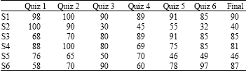 | |
| Column means quiz score, S1-S8 means specific course | |
| Table 2: | Transfer record contrasting |
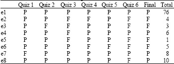 | |
| P: Pass, F: Failure | |
Did not pass the final exam in this course means that did not pass. Therefore, the main issue is, which part of the students lack understanding of the content (i.e., no small achievement tests passed) led to their final exam fail. We can use a table of information to determine (Liang et al., 2000) the final grade is not good cause the relevant rules. In the future so that we can tell the students the teaching of courses in a central part and hence the appropriate guidance to students.
The following is a quiz about the students and the final examination of the text file. Including 115 students, 6 quizzes and a final exam (Table 1).
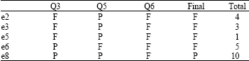
First, we only care about the students in this course is passed, so we can convert out this form, the table P that pass, F, said failure. Students in the same situation and put into one category which are at a simple table, a total of eight categories, not difficult to find, in the total number of students into a 113, the other two in each quiz are not passed students, we are not considered because of their logical end result should be a Failure (Table 2). In Table 2, P stands for pass, F stands for failure, “e” stands for the number of exam.
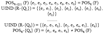
Reduction, which requires reduction of redundant information out, in order to achieve this step, we use linear searching and sorting methods to complete. In the table above, for example, the table R = {Q1, Q2, Q3, Q4, Q5, Q6, Final}
R positive domain is:
POSR (F) = {e1, e2, e3, e4, e5, e6, e7, e8} |
To calculate the reduction on, we need to study whether it is-independent.
| Table 3: | Simplify data contrasting |
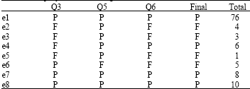 | |
| P: Pass, F: Failure | |
When we used to test the removal of circulating were the positive field, if every time a small test field is not equal to the final exam is the positive region, we reserve the condition attributes, the following is a partial result of the operation:
 |
We conclude from the above operation: e3, e5, e6 is essential, because it is not equal to the Final of the domain is the domain. Further, we have simplified information Table 3.
The remaining work is to find decision rules. We have the following results On the field:
| • | Failure category: Y = {e2, e3, e5, e6} |
| • | Based on the non-recognition category Quiz: |
| • | Lower approximation Y = {} |
| • | Upper approximation |
| • | Identify indicators: |
Calculated the same Q5, Q6 index, we get the right table.
We calculate the α exponentiate and get the right Table 4.
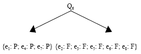
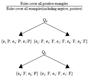
It can be seen Quiz 6 value is the highest recognition that is it is a member of the best decisions in the areas Y, therefore, To the following decision rules we have:
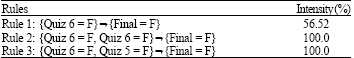
Rule1: {Quiz 6 = F} ⇒ {Final = F} |
The resulting decision tree is as follows:
| Table 4: | Data contrasting |
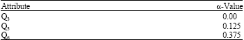 | |
| Column means quiz attribute, α Value means sampling results | |
| Table 5: | Record contrasting based on the decision tree |
 | |
| P: Pass, F: Failure | |
 |
We have been based on decision tree. See also Table 5.
Then we combine with the remaining condition attributes to find the highest recognition of the financial indicator, thus creating two combinations, the right table is the result of the second round of calculations.
Then we combine Q6 with the remaining condition attributes to find the highest recognition of the financial indicator, thus creating two combinations Q6, Q3 and Q6, Q5, the right table is the result of the second round of calculations:
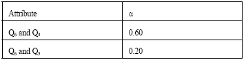 |
Not difficult to see Q6 and Q3 from the table, with a high recognition index, we get:
The second Rules:
Rule 2: {Quiz 6 = F, Ouiz 3 = F} ⇒ {Final = F} |
Combination of decision tree as shown on page Table 1.
Using the same method we can get:
Rule 3: {Quiz 6 = F, Ouiz 5 = F} ⇒ {Final = F} |
Over the course of our out of the rules for online students is concerned, these rules have little credibility it? The concept of classification of intensity answered this question, it could use the formula to calculate the:
 |
In order to calculate the final step, we again used the line search, the rule strength calculation table below (Table 6).
Table 6 can be summarized as follows: If a student does not pass the quiz, then he will have a 56.52% final exam can not be possible. If an online learning and the students did not pass the exam Quiz 6 and Quiz 5, then he can not say 100% pass the final exam. This form of online is learned by the students before the performance analysis, for the later study the same course provides guidance for students.
DECISION-MAKING ROLE IN MEDICAL DIAGNOSIS
Molodtsov (1999) proposed soft set theory to solve the problem of uncertainty, a common method and its non-binding parameters, improving the practical application of the decision problem. It is defined as follows:
Definition 1: U is the initial domain of, E is Parameter set,then (F, E) is U On the soft set if and only if F is from E to U a map of all subsets.
For any ε∈E , eavh F (ε) can be seen as a soft set (F, E) each ε has one element. Soft collection of parameter settings without any constraints, the elements can be words, sentences, equations and even functions, mapping. Some of the definitions on rough sets can be defined in parallel over. Consider the soft set (F, E), P ⊂ E, (F, P) is (F, E) a subset of soft set, Now according to the definition of rough sets to define reduction of soft set, respectively and the nuclear soft set. If Q is P reduction, then soft set (F, Q) is soft set (F, P) the reduction of soft sets, if C is P’s shore, then soft set (F, C) is (F, P) nuclear soft set.
Maji et al. (2002) have used a soft set to make home buying decision problem, also in the clinical diagnosis, we can also do the decision-making problems with soft set. For Table 1, the initial universe is to be considered in all cases, the parameter set is a collection of all of the symptoms.
| Table 6: | Intensity computation |
 | |
Definition of soft set for this problem which is that the symptoms were characteristic of a certain set of cases. We focused on the actual clinical diagnosis; the which is defined as the classification accuracy of the weight of the medical diagnosis of some decision-making to do some improvements.
First, the use of soft non-binding set of parameters, we put into a Table 1, 0/1 Truth table, this representation is very suitable for computer storage of a soft set. Changes as follows: if ui ∈ F(ε), then uij =1, then uij = 0, uij that is Table 1 is truth table. Thus, We get from Table 1, Table 2, Table 3 Two truth tables. Calculation of each rule-each atomic formula R accuracy of decision-making αR, That is, with a probability of disease after the symptoms D, so that after the algorithm by induction:
| • | Input soft set (F, E) |
| • | Enter the diseases to be investigated will be used by the collection of all the symptoms, namely, E subset P |
REDUCTION IDENTIFIED BY MATRIX PROPERTIES
General reduction algorithm is a process of exhaustive search, the time complexity of a great need, therefore, the introduction of the discernibility matrix method.
Definition 2: Decision table system S = < U, R, V, f ,>, R = P ∪ D is the attribute set, subset D = {d} and P = {ai| i = 1, 2,...,m} are decision attributes and condition attributes, U = {x1, x2,..., xn } on the field, ai (xj)is the sample xj in the Properties ai the value, CD (i, j) discernibility matrix that i line j column element, then Matrix can be identified CD defined as follows:
Nuclear is the discernibility matrix elements in the collection of the entire individual, that:
Core (A) = {aεA|a(x, y) = {a}, x, y,ε U} |
Based on discernibility matrix attribute reduction algorithm is summarized as follows:
| • | The calculation of the discernibility matrix of decision table CD |
| • | The matrix can identify all the elements of the value of non-empty set Cij, Establish the appropriate expression of disjunctive logic |
| • | The expression of all disjunctive Lij the conjunctive operation, Be a CNF L, namely, |
| • | The CNF L is converted to disjunctive normal form |
| • | Disjunctive conjunction of each item is the result of a reduction |
In fact this algorithm is to attribute combinations in the search into a logical formula simplification.
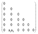
For example, Table1 Discernibility matrix corresponding to:
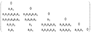 |
Individual elements of which a2, a3 is kernel.
So we got 15 DNF:
 |
| • | The conjunction of their operation, get a conjunctive normal form: |
For L make Conversion, Finally get L' (a1∧a2∧a3)∨(a2∧a3∧a5).
So, are the two set of attributes reduction {a1, a2, a3} and {a2, a3, a5}.
This is actually a logical process of simplifying the formula, because the extract obtained by the matrix formula, namely Lij number will increase as the surge in the sample, so we need some changes in the following.
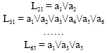
Discernibility matrix to see if there is a matrix element, its value as a collection of elements containing a single attribute, then that attribute to distinguish between the matrix elements corresponding to the attributes necessary for the two samples, the properties can be distinguished only can identify these elements in a matrix composed of multi-attribute contains a collection of attributes, in fact, the decision table system, the relative properties of nuclei. So we can remove these attributes first, and will contain elements of the property value of the nuclear correction to 0 to have a new matrix, and then run the algorithm the first step by 2, 3, 4, 5-disjunction. Matrix from above, we can identify the matrix contains all the elements by a single attribute to 0, the original matrix into:
 |
Then, L' = a1∨a5, appended a2, a3, been (a1∧a2∧a3)∨(a2∧a3∧ a5)
Then, {a1, a2, a3} and {a2, a3, a5} is a reduction of the original property.
CONCLUSION
In this study, the rough set algorithm implementation of distance education, distance education issues to improve the feedback problem. In this paper, the conclusions apply not only to distance learning on the Internet, but also for practice, teaching, and to give new teachers a large extent the teaching reference.
REFERENCES
- Hongyan, G. and B. Maguire, 2003. A rough set methodology to support learner self-assessment in web-based distance education. Rough Sets Fuzzy Sets Data Mining Granular Comput., 2639: 582-582.
CrossRef - Wong, S.K.M., W. Ziarko and R.L. Ye, 1986. Comparison of rough-set and statistical methods in inductive learning. Int. J. Man-Machine Stud., 24: 53-72.
CrossRef - Liang, A.H., B. Maguire and J. Johnson, 2000. Rough set based webCT learning. Proceedings of the 1st International Conference on Web-Age Information Management, June 21-23, Springer-Verlag, Berlin, Heidelberg, pp: 425-436.
Direct Link - Wei, W., A. Gao, B. Zhou and Y. Mei, 2010. Scheduling adjustment of mac protocols on cross layer for sensornets. Inform. Technol. J., 9: 1196-1201.
CrossRefDirect Link - Wei, W., B. Zhou, A. Gao and Y. Mei, 2010. A new approximation to information fields in sensor nets. Inform. Technol. J., 9: 1415-1420.
CrossRefDirect Link - Maji, P.K., A.R. Roy and R. Biswas, 2002. An application of soft sets in a decision making problem. Comput. Math. Appl., 44: 1077-1083.
CrossRef - Gao, A., W. Wei and X. Xiao, 2010. Multiple hash Sub-chains: Authentication for the hierarchical sensor networks. Inform. Technol. J., 9: 740-748.
CrossRef - Wei, W., Y. Qi, S. Qi, D. Hou, W. Wang, M. Xi and Q. Yao, 2007. Energy efficient multi-rate based time slot pre-schedule scheme in WSNs for ubiquitous environment. Proceedings of the IEEE Computer Society Asia-Pacific Services Computing Conference, Dec. 11-14, IEEE Computer Society, Washington, DC. USA., pp: 75-80.
- Wei, W., Y. Qi, X. He, W. Wang, R. Li and H. He, 2008. Improving the survivability of WSNs with biological characters based on rejuvenation technology. Proceedings of the 2008 IEEE Asia-Pacific Services Computing Conference, Dec. 9-12, IEEE Computer Society Washington, DC., USA., pp: 644-649.
CrossRef - Wei, W., Y. Qi, W. Wang, R. Li, Y. Shi, Y. Gu and A. Chen, 2008. Variant rate based cross layer time frame scheduling in wireless sensor networks. Proceedings of the 7th Annual Wireless Telecommunications Symposium, April 24-26, IEEE Communication Society, Cal Poly Pomona, California, USA., pp: 62-68.
CrossRef - Wei, W., S. Qi, Y. Qi, W. Wang and M. Xi, 2007. Allotropy programming paradigm for ubiquitous computing environment. Proceedings of the IEEE Computer Society International Conference on Convergence Information Technology, Nov. 21-23, IEEE Computer Society, Washington, DC, USA., pp: 514-521.
CrossRef - Gao, A., W. Wei, Z. Wang and Y. Wenyao, 2009. A hierarchical authentication scheme for the different radio ranges sensor networks. Proceedings of the 7th IEEE/IFIP International Conference on Embedded and Ubiquitous Computing, Aug. 29-31, Vancouver, Canada, pp: 494-501.
CrossRef