
Malik Sikander Hayat Khiyal
Fatima Jinnah Women University, The Mall, Rawalpindi, Pakistan
Journal of Applied Sciences
Year: 2008 | Volume: 8 | Issue: 2 | Page No.: 252-261


ABSTRACT
A family of sixth order and fourth order P-stable methods for solving second order initial value problems is considered. The nonlinear algebraic systems, which results on applying one of the methods in this family to a nonlinear differential system, may be solved by using a modified Newton method. The local error estimation technique based on the derivation of suitable formula pairs is used in which we compute two approximations of the solution, one with a fourth order method and the other with a sixth order method. The error estimate is then obtained by subtracting our two approximations. The methods in each pair are chosen to have certain features in common. They have the same iteration matrix and some of the function evaluations are common to both methods. Finally numerical results are presented of these methods.
PDF Abstract XML References Citation
How to cite this article
Malik Sikander Hayat Khiyal, 2008. Sixth Order/Fourth Order P-Stable Methods for Second Order Initial Value Problems. Journal of Applied Sciences, 8: 252-261.
DOI: 10.3923/jas.2008.252.261
URL: https://scialert.net/abstract/?doi=jas.2008.252.261
DOI: 10.3923/jas.2008.252.261
URL: https://scialert.net/abstract/?doi=jas.2008.252.261
INTRODUCTION
We consider the class of direct hybrid methods proposed by Cash (1981) then extended by Khiyal (1991) for solving the second order initial value problem.
(1) |
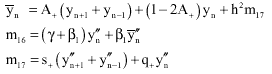
The basic methods has the form
(2) |
Where:
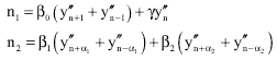
The off-step values are defined by
(3) |
(4) |
![]()
and
When the method (2-4) is applied to a nonlinear differential system (1), a nonlinear algebraic system must be solved at each step. This may be solved by using a modified Newton iteration scheme. The resulting iteration matrix involves J, J2 and J3, where J is an approximation for the Jacobian matrix of f with respect to y. Since matrix products are expensive, especially for large systems and any sparsity in J will be weakened in J2 and J3 and any ill-conditioning in J will be magnified in its powers, we wish to avoid the calculation of J2 and J3. Cash (1981), Thomas (1988), Khiyal (1991) and Khiyal (2007b) have derived sixth order P-stable (Lambert and Watson, 1976) methods of the form (2-4) for which the iteration matrix is a true perfect cube.
By taking β2 = 0 in (2) and choosing the remaining parameters appropriately, several authors (Cash, 1981; Chawla, 1981; Chawla and Neta, 1986; Costabile and Costabile, 1982; Khiyal, 1991; Thomas, 1988; Khiyal, 2007a) have derived fourth order methods of the form (2-4) which are P-stable.
The present consider the fourth order method of Thomas (1987), Khiyal (1991) and Khiyal (2007a) and sixth order methods of Thomas (1988), Khiyal (1991) and Khiyal (2007b).
We give necessary and sufficient conditions for there to exit
| • | Fourth order, P-stable, two-evaluations, two-step methods with iteration matrix (I-rh2J)2 |
| • | Sixth order, P-stable, three-evaluations, two-step methods with iteration matrix (I-rh2J)3 |
The method may be chosen so that the value of r is the same for both the fourth and sixth order methods. We derive some formula pairs. (The formula pair technique discussed by Khiyal (1991) and Khiyal and Thomas (2006).
MATERIALS AND METHODS
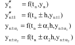
The modified Newton iteration scheme for methods of the form (2-4) is given by:
(5) |
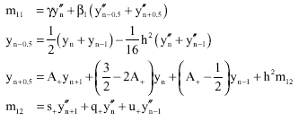
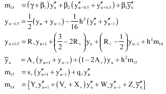
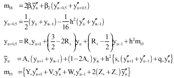
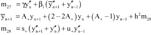
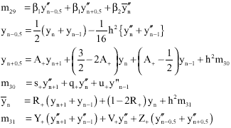
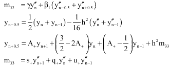
For sixth order methods as defined by Khiyal (2007b)
(6) |
Where: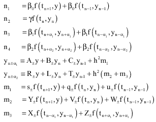
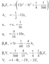
and
(7) |
To avoid the calculation of J2 and J3 Thomas (1988) and Khiyal (1991) has shown that the iteration matrix (5) may be factorized as a true perfect cube
![]()
Where:
![]()
The necessary and sufficient conditions for this are
(8a) |
(8b) |
The resulting methods are P-stable if and only if
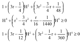 | (9) |
hold for all H. These conditions are satisfied when r is greater than or equal to the largest real root of the polynomial equation
(10) |
Note that the largest root of (10) is r = 0.6564 to four significant figure. Then the iteration scheme (5) has the form
(11) |
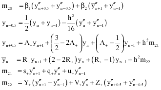
The Newton iteration scheme for fourth order methods of the form (2-4) with β2 = 0 is given by
(12) |
Where: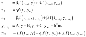
and
(13) |
A true perfect square iteration matrix is
![]()
Where:
![]()
For the fourth order methods, this is the case if and only if
(14) |
and the resulting methods are then P-stable if and only if
(15) |
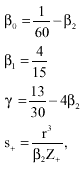
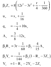
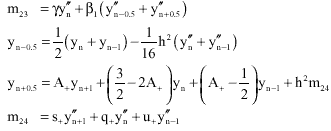
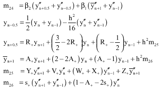
Derivation of formula pairs: The three evaluations P-stable, sixth order methods of the type given by Thomas (1988), Khiyal (1991), Khiyal and Thomas (2006) and Khiyal (2007b) may be combined in a variable step code with appropriate two evaluations P-stable fourth order methods of the type given by Thomas (1987), Khiyal (1991) and Khiyal (2007a). The iteration matrix for the sixth order methods is![]() where, to ensure P-stability
where, to ensure P-stability![]() and R is the largest root of the polynomial (10). The iteration matrix for the fourth order method is
and R is the largest root of the polynomial (10). The iteration matrix for the fourth order method is![]() where
where
![]()
for P-stability. For common iteration matrix we choose r >=R. The local error estimate is given by
![]()
Where, ![]() is the approximation for y(tn+1) obtained by the method of order 2m, m = 2 and 3. The different formula pairs are:
is the approximation for y(tn+1) obtained by the method of order 2m, m = 2 and 3. The different formula pairs are:
SHK64A: The sixth order method is the method given by Khiyal (1991) and Khiyal (2007b) for which ![]() is independent of yn+1 and the points
is independent of yn+1 and the points![]() are coincident. For this method we must evaluate
are coincident. For this method we must evaluate![]() once per step. With this sixth order method, we combine a fourth order method given by Khiyal (1991) and Khiyal (2007a) such that
once per step. With this sixth order method, we combine a fourth order method given by Khiyal (1991) and Khiyal (2007a) such that![]() is independent of yn+1 and
is independent of yn+1 and ![]() need only be evaluated once per step. Note that
need only be evaluated once per step. Note that![]() has to be evaluated once per step for each of the fourth and sixth order methods. We choose α1 to be the same for both methods and we also choose the coefficients in the expression (3) to ensure that
has to be evaluated once per step for each of the fourth and sixth order methods. We choose α1 to be the same for both methods and we also choose the coefficients in the expression (3) to ensure that ![]() is the same for both methods. This means that
is the same for both methods. This means that ![]() must be evaluated just once per step and may then be used for both the fourth and sixth order methods.
must be evaluated just once per step and may then be used for both the fourth and sixth order methods.
Sixth order method:
(16) |
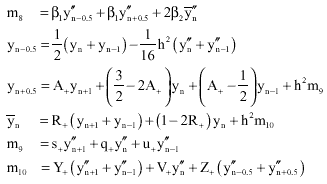
Where: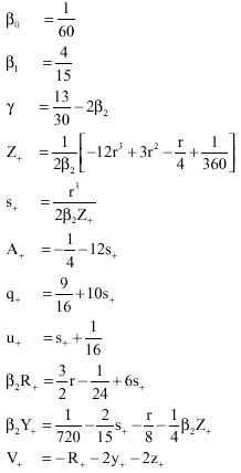
β2 is free parameter (we choose β2 = 1).
Fourth order method
(17) |
Where: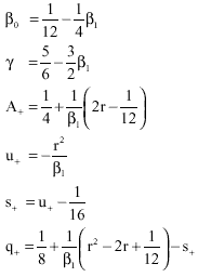
β1 is free parameter (we choose β1 = 1).
r is greater than or equal to the largest root of the cubic Eq. 10 for both sixth and fourth order methods.
SHK64B: The sixth order method is the method given by Khiyal (1991) and Khiyal (2007b) for which![]() is identically equal to
is identically equal to![]() and
and![]() is independent of yn+1. For this method we must evaluate
is independent of yn+1. For this method we must evaluate ![]() once per step. We combine this method with a fourth order method given by Thomas (1987), Khiyal (1991) and Khiyal (2007a), for which
once per step. We combine this method with a fourth order method given by Thomas (1987), Khiyal (1991) and Khiyal (2007a), for which![]() is identically equal to.
is identically equal to.
Sixth order method
(18) |
Where: 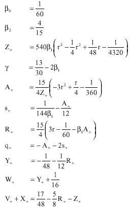
β1 are free parameters.
Fourth order method
(19) |
Where: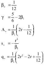
β1 are free parameters.
r is greater than or equal to the largest root of the cubic Eq. 10 for both the sixth and fourth order methods.
SHK64C: Consider the sixth order method given by Khiyal (1991) and Khiyal (2007b) for which the points![]() are coincident and
are coincident and ![]() is independent of yn+1. For this method we must evaluate
is independent of yn+1. For this method we must evaluate ![]() once per step. We combine the method given by Thomas (1987), Khiyal (1991) and Khiyal (2007a) for which the points
once per step. We combine the method given by Thomas (1987), Khiyal (1991) and Khiyal (2007a) for which the points![]() are coincident.
are coincident.
Sixth order method
(20) |
Where: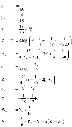
β1 are free parameters.
Fourth order method
(21) |
![]()
Where: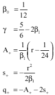
β1 are free parameters.
r is greater than or equal to the largest root of the cubic Eq. 10 for both the sixth and fourth order methods.
SHK64D: Consider the sixth order given by Khiyal (1991) and Khiyal (2007b) for which ![]() is independent of yn+1 and
is independent of yn+1 and ![]() . For this method we need to evaluate
. For this method we need to evaluate ![]() once per step. We combine fourth order method given by Khiyal (1991) and Khiyal (2007a) such that
once per step. We combine fourth order method given by Khiyal (1991) and Khiyal (2007a) such that![]() is independent of yn+1. This means that
is independent of yn+1. This means that ![]() must be evaluated just once per step and may be used for both fourth and sixth order methods.
must be evaluated just once per step and may be used for both fourth and sixth order methods.
Sixth order method
(22) |
Where:
β2 are free parameters.
Fourth order method
(23) |
Where: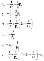
β1 is free parameter.
r is greater than or equal to the largest root of the cubic Eq. 10 for both sixth and fourth order methods.
SHK64E: Consider the` sixth order method given by Khiyal (1991) and Khiyal (2007b) for which![]() is identically equal
is identically equal ![]() to and is independent of yn+1. For this method we need to evaluate
to and is independent of yn+1. For this method we need to evaluate ![]() once per step. We combine this method with a fourth order method given by Thomas (1987), Khiyal (1991) and Khiyal (2007a).
once per step. We combine this method with a fourth order method given by Thomas (1987), Khiyal (1991) and Khiyal (2007a).
Sixth order method
(24) |
Where: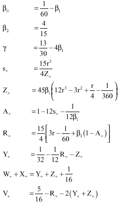
β1 are free parameter.
Fourth order method
(25) |
Where: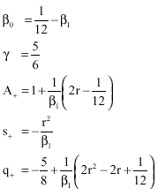
β1 is free parameter.
r is greater than or equal to the largest root of the cubic Eq. 10 for both sixth and fourth order methods.
SHK64F: Consider the sixth order method given by Khiyal (1991) and Khiyal (2007b) for which is ![]() independent of yn+1 and
independent of yn+1 and ![]() . For this method we need to evaluate
. For this method we need to evaluate![]() once per step. We combine this method with a fourth order method given by Khiyal (1991) and Khiyal (2007a) for which
once per step. We combine this method with a fourth order method given by Khiyal (1991) and Khiyal (2007a) for which![]() is independent of yn+1. This means that
is independent of yn+1. This means that ![]() must be evaluated once per step and may be used for both fourth and sixth order methods.
must be evaluated once per step and may be used for both fourth and sixth order methods.
Sixth order method
(26) |
Where:

β2 is free parameter.
Fourth order method
(27) |
Where: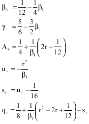
β1 is free parameter.
r is greater than or equal to the largest root of the cubic Eq. 10 for both sixth and fourth order methods.
RESULTS
We are mainly concerned with solving oscillatory stiff initial value problem. We have tried a number of explicit scalar (nonstiff) test problems of the form (1). They give similar results and so we restrict our attention to one oscillatory example.
Example 1:
This is a pure oscillation problem whose solution has maximum amplitude unity and period approximately six. We have calculated error as |Error at t = 6|
To verify that our techniques works for systems, we use a test problem a moderately stiff system of two equations
Example 2:
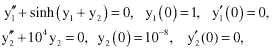 |
For this example we have deliberately introduced coupling from the stiff (linear) equation to the nonstiff (nonlinear) equation. For this example again we have calculated error as![]() .
.
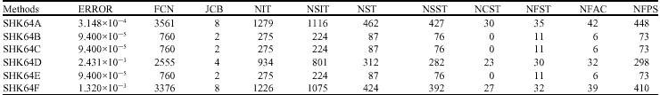
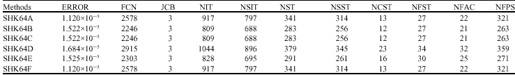
In Table 1-6, we present the following statistics:
| • | No. of evaluation of the differential equation right hand side f, FCN |
| • | No. of evaluation of the Jacobian |
| • | No. of iteration overall, NIT |
| • | No. of iteration on steps where the iteration converges, NSIT |
| • | No. of steps overall, NST |
| • | No. of successful steps to complete the integration, NSST |
| • | No. of steps where the stepsize is changes, NCST |
| • | No. of failed steps, NFST |
| • | No. of LU factorization of the iteration matrix, NFAC |
| • | No. of function evaluation required on a per step basis, rather than on each iteration, NFPS |
The results are given in Table 1-6. The cost of the starting technique is not included in the tables. Before we can employ this error estimation technique, we need a special starting technique to obtain the values y1 and y2. Thus we take two steps with fourth order, two stages Implicit Runge Kutta method. The technique used is given by Khiyal and Rashid (2005). After two steps we use the formula pair technique. After word at the end of each step, we form the error estimate Len+1. To estimate the local error we use predictor corrector approach. For predictor we use the polynomial of degree five given by Khiyal (1991).
If the local error is satisfied, we use the sixth order direct hybrid method. At the each step, we form the error estimate;
Where, is the approximation for y(tn+1) obtained by the method of order 2m, m = 2 and 3. The step size for the next step is given by:
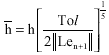 |
Where![]() , Tol is the local error tolerance and h is the current step size and is the next predicted step size
, Tol is the local error tolerance and h is the current step size and is the next predicted step size![]() . We do not allow the step size to decrease by more than a factor ρ1 or increase by more than a factor ρ3. These restrictions help to avoid large fluctuation in the step size caused by local changes in the error estimate. Also, we do not increase the step size at all unless it can be increased by a factor of at least ρ2, where ρ2<ρ3. This restriction is designed to avoid the extra function and Jacobian evaluation involved in changing the step size unless a worthwhile increase is predicted. Following Thomas (1987), in our tests we take ρ1 = 0.1, ρ2 = 2 and ρ3 = 10.
. We do not allow the step size to decrease by more than a factor ρ1 or increase by more than a factor ρ3. These restrictions help to avoid large fluctuation in the step size caused by local changes in the error estimate. Also, we do not increase the step size at all unless it can be increased by a factor of at least ρ2, where ρ2<ρ3. This restriction is designed to avoid the extra function and Jacobian evaluation involved in changing the step size unless a worthwhile increase is predicted. Following Thomas (1987), in our tests we take ρ1 = 0.1, ρ2 = 2 and ρ3 = 10.
| Table 1: | Methods are compared for example 1 with Tol = 10-2 |
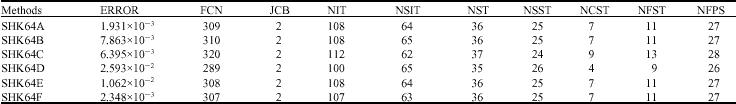 | |
| Table 2: | Methods are compared for example 1 with Tol = 10-4 |
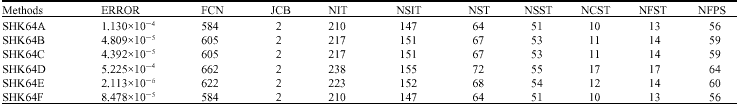 | |
| Table 3: | Methods are compared for example 1 with Tol = 10-6 |
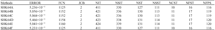 | |
| Table 4: | Methods are compared for example 2 with Tol = 10-2 |
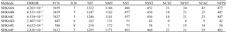 | |
| Table 5: | Methods are compared for example 2 with Tol = 10-4 |
 | |
| Table 6: | Methods are compared for example 2 with Tol = 10-6 |
 | |
CONCLUSIONS
In the study, we have derived some formula pairs, consisting of a fourth order and a sixth order direct hybrid method. The two methods in each pair have been chosen to have some features in common, so that the computational cost of using the formula pair is reduced. The formula pairs provide an estimate of the local error and this allows the stepsize to be varied so that the size of the local error is controlled.
REFERENCES
- Cash, J.R., 1981. High order P-stable formulae for the numerical integration of periodic initial value problems. Numer. Math., 37: 355-370.
CrossRefDirect Link - Chawla, M.M., 1981. Two step fourth order P-stable methods for second order differential equations. BIT Numer. Math., 21: 190-193.
CrossRefDirect Link - Chawla, M.M. and B. Neta, 1986. Families of two-step fourth order P-stable methods for second order differential equations. J. Comput. Applied Math., 15: 213-223.
CrossRefDirect Link - Costabile, F. and C. Costabile, 1982. Two-step fourth order P-stable methods for second order differential equations. BIT Numer. Math., 22: 384-386.
CrossRefDirect Link - Khiyal, M.S.H. and K. Rashid, 2005. Implementation of s-stage Implicit Runge-Kutta methods of order 2s for second order initial value problems. J. Applied Sci., 5: 411-427.
Direct Link - Khiyal, M.S.H. and R.M. Thomas, 2006. Eighth order/sixth order methods for second order initial value problems. Inform. Technol. J., 5: 803-812.
CrossRefDirect Link - Khiyal, M.S.H., 2008. Sixth order/fourth order p-stable methods for second order initial value problems. J. Applied Sci., 8: 252-261.
CrossRefDirect Link - Khiyal, M.S.H., 2007. Efficient sixth order P-stable methods for second order initial value problems. J. Applied Sci., 7: 3592-3605.
CrossRefDirect Link - Lambert, J.D. and I.A. Watson, 1976. Symmetric multistep methods for periodic initial value problems. IMA J. Applied Math., 18: 189-202.
CrossRefDirect Link - Thomas, R.M., 1988. Efficient sixth order methods for nonlinear oscillation problems. BIT Numer. Math., 28: 898-903.
CrossRefDirect Link