
Prabeer Kumar Parhi
Center for Water Engineering and Management, Central University of Jharkhand, 835205 Brambe, India
LiveDNA: 91.16228
International Journal of Agricultural Research
Year: 2017 | Volume: 12 | Issue: 3 | Page No.: 115-122


ABSTRACT
Background and Objective: Border strip method of irrigation is a widely used surface irrigation technique which is best adapted to crops like wheat, barley, fodder crops and legumes. The present study was aimed to design an irrigation border to maximize water application efficiency which is very important to meet the growing water needs. Materials and Methods: Using the modified water front advance-time relation, an irrigation border has been designed and its efficiency was evaluated. The derived design procedure ensured application of uniform depth of irrigation throughout the length of border thus maximizing water application efficiency of the irrigation borders. In the present study the required optimum border length, entrance stream size and the corresponding Manning’s ‘n’ had been derived to achieve optimum irrigation water application efficiency. The derived design procedure has been applied to the wheat crop cultivated in sandy loam soil in the Ramiala irrigation command (Orissa, India) to determine entrance stream size and corresponding optimum border length. Results: The result of the study showed that the optimum border length and entrance stream size required are, respectively 40 m and 2906 cm3 min–1 cm–1 which gives maximum water application efficiency up to the tune of 83.32%. Conclusion: The modified design technique increases the water application efficiency of the irrigation borders, which appears very high as compared to the achieved efficiency of 66.5%, as available in the literature. The suggested method appears very simple and can be applied easily to crops having different root zone depths cultivated in different soils.
PDF Abstract XML References Citation
Received: March 14, 2017;
Accepted: May 15, 2017;
Published: June 15, 2017
How to cite this article
Prabeer Kumar Parhi, 2017. Improving Water Application Efficiency of Irrigation Borders Using Modified Water Front Advance-time Relation. International Journal of Agricultural Research, 12: 115-122.
DOI: 10.3923/ijar.2017.115.122
URL: https://scialert.net/abstract/?doi=ijar.2017.115.122
DOI: 10.3923/ijar.2017.115.122
URL: https://scialert.net/abstract/?doi=ijar.2017.115.122
INTRODUCTION
The border-strip method of surface irrigation is a widely used irrigation technique which is best adapted to crops like wheat, barley, fodder crops and legumes, where topography is flat1. The design of border irrigation requires many input parameters and needs extensive engineering calculations and therefore, the experimental trial and error design is frequently resorted to Khanjani and Barani2. A border irrigation system is designed for entrance stream size, the length of run or slope of the border in such a way that it can replenish the soil moisture in the root zone uniformly before it depletes beyond a specific limit. To derive the maximum application efficiency, the water is allowed to stay on the surface for a sufficiently long time to permit the desired amount of water to infiltrate into the soil1. It is important to mention that in an existing field layout, the length or slope of the border cannot be altered and the entrance stream size forms to be the main controllable variable that can be designed to increase the efficiency of the system.
The study of surface irrigation system can be classified into two basic categories, namely design and analysis. While determination of water front advance with time is an analysis problem, computation of optimum stream size, to achieve maximum irrigation efficiency is a design problem. The analysis of flow in surface irrigation is complex due to the interactions of several variables such as infiltration, inflow rate and hydraulic roughness3. The design, however, is more complex due to interactions of these input variables and the involved output parameters like efficiencies, uniformities, deep percolation and runoff4.
The efforts in analysis and design of surface irrigation have predominated during last few decades. The studies of previous researchers5-11 are only a few to cite among many others. The design of surface irrigation is however has been summarized in a few reports only. For example, Hall12 developed a design procedure based on the calculation of rate of advance from the observed or expected infiltration characteristics, allowable range of slope, possible value of roughness and maximum allowable stream size, which was further modified and simplified by Michael1. The Soil Conservation Service13 developed a design procedure for several types of surface irrigation systems. Walker and Skogerboe14 proposed a design procedure for graded borders, furrows and basins. Clemmens et al.15 developed a dimensionless solution for level basin design. Using Kostiakov infiltration model, Alazba,4 presented a border design, applicable to sloping open-ended borders only. Khanjani and Barani2 proposed a system-based border irrigation design technique using border irrigation storage and distribution efficiencies, border slope and length, inflow rate, cutoff time and Manning’s roughness coefficient as constraints.
Using the water front advance-time relationship, Michael and Pandya7 and Michael1 modified the design procedure suggested by Hall9. However, the complexity of equations used for the determination of water front advance-time relation makes the existing design procedure more complex and less popular. In view of the above, the present study attempts to modify and simplify the Michael’s1 design procedure using water front advance-time relation which does not appear to have been reported in literature. Thus, the objective of the current study was to further modify the Michael’s1 technique for the design of the irrigation borders applying the water front advance-time relations of Parhi16 derived using kostiakov (KT)17, modified kostiakov (MKT)18 and improved modified kostiakov (IMKT)19 infiltration models.
MATERIALS AND METHODS
Study area: The present study was carried out and applied to the field data of Ramial irrigation command (Orissa, India). The climate of the study area is tropical with fairly hot summer, moderately cold winter and humid rainy season. The temperature of the area varies from a minimum of 12.9°C to a maximum of 39.9°C having average annual rainfall as 1182 mm. The rainfall is confined from June-October during which 90% of annual rainfall is received. The rainfall received in rest of the period is of no agro-irrigational interest as much of it is lost in infiltration and evaporation. As border irrigation system is most suited for the wheat crop, which is largely cultivated during Rabi season, a border irrigation system is designed using the field data and applied to this area to achieve maximum irrigation efficiency.
Data used: Due to non-availability of infiltration data of the study area, which is essential for the design of a border irrigation system, the data employed here is taken from the infiltration tests carried out by Michael20, on sandy loam soil (same to the study area). The data has been used to determine the functional form of y (t). The field capacity and wilting point of the sandy loam soil in study area have been considered as 16 and 4%, respectively21, thus making the water holding capacity of soil as 12% (12 cm m–1 depth). The root zone depth of wheat crop has been taken as 1-1.5 m and average being 1.25 m22.
Parameter estimation of infiltration data: To find the equation of a specified type that best fits the set of observations, the optimal values of parameters of various infiltration models i.e. KT, MKT and IMKT, were estimated using the method of least squares. The method suggests that, for the best fits, the sum of the squares of differences between the observed and the corresponding estimated values are minimum23, which can be expressed as:
| (1) |
where, Z is the error, N is the number of observations or times, fobs (i) is the observed infiltration rate at ith time and fcom(i) is the computed infiltration rate at ith time.
In this study, the software package, Language for Interactive General Optimizer (LINGO) was used to minimize the errors. The accumulated infiltration-time relationship, using the infiltration data for the soil type in question, resulting from the employment of above mentioned models, exhibited a form as y = 1.459t0.697. This appears to be in the form KT, where y equals accumulated infiltration at any time t.
Performance evaluation: Among the several statistical measures available for evaluating the performance of a model, such as correlation coefficient, relative error, standard error etc., the Nash and Sutcliffe24 efficiency is most frequently used23 and it has been employed in this study.
The efficiencies resulting from the employment of KT, MKT and IMKT models to infiltration data in a wheat field in predicting accumulated infiltration-time relationship, performed identically and yielded 99.9% efficiency value, exhibiting a more than satisfactory performance.
Water front advance-time relation: As KT, MKT and IKMT showed identical results in predicting the accumulated infiltration-time relationship, the water front advance-time relationship is computed using KT, because it provides the simplest form of water front advance-time relationship, converges satisfactorily and rapidly for almost all values of t giving satisfactory results19. In the context of present discussion it is pertinent to present here the water front advance-time relationship using KT which forms the most important component in design of border irrigation system19, which can be written as:
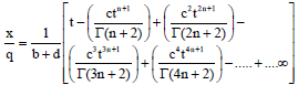 | (2) |
and
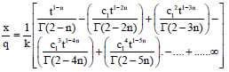 | (3) |
where, q is the constant rate of flow per unit width introduced at the upstream end of the border (cm2 min–1 cm–1 width of border), t is the total time for which irrigation water has been applied (min), x is the distance, the irrigation stream has advanced in time’t’ (cm), d is the average depth of flow over the ground surface (cm):
![]()
and m, n and b are infiltration parameters determined by optimization. The Eq. 2 and 3 works best for small and large values of t, respectively.
RESULTS AND DISCUSSION
Design of border irrigation system: The depth of water required to replenish the soil moisture in the root zone to field capacity is calculated as the product of water holding capacity and average depth of root zone (15 cm in the present study). Considering different possible values of stream size (q) as 3000, 3200, 3400 and 3600 cm3 min–1 cm–1 width, the approximate values of Manning’s roughness ’n’ is calculated using equation1 as:
| (4) |
where, v is the velocity (m sec–1), R is the hydraulic radius (m) s is the soil surface slope (%). The values of Manning’s’ n’ computed using Eq. 4 for a vegetated (wheat crop) field having sandy loam soil are 0.257, 0.256, 0.255 and 0.254, respectively for stream sizes 3000, 3200, 3400 and 3600 cm3 min–1 cm–1 width.
Using the values of ’q’ and ’n’, the depth ’do’ at the upstream end of the border is calculated1 as.
| (5) |
where, q is the entrance stream size.
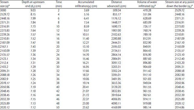
| Table 1: | Calculation procedure for the estimation of average depth of flow (d) for ’q’ and ’do’ of 3000 cm3 min–1 cm–1 and 9.03 cm, respectively |
 | |
| *Unit cm3 min–1 cm–1 | |
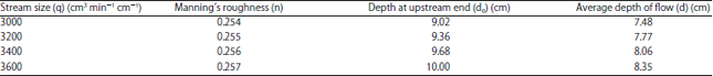
| Table 2: | Values of ’n’ and ’do’ for different values of ’q’ under consideration |
 | |
Further, the flow depths d1, d2, d3.... dn at successive points along the border is calculated by considering the distance advanced at equal time increments using water front advance-time relation (Eq. 2, 3) and its average is taken as d. The water depth required at successive points down the border will decrease as the total flow along these points decrease. Hence the water depth is a function of the distance down the border. Thus the stream size (qo), at any point down the border equals the difference between the entrance stream size (q) and the average rate of the volume of water (qi) infiltrated over the area from the upstream of border.
In the present study considering the value of ’q’ as 3000 cm3 min–1 cm–1 the approximate value of ’n’ is estimated (using Eq. 4) as 0.257 for a wheat field. Subsequently using ’q’ and ’n’ as 3000 cm3 min–1 cm–1 and 0.257, the depth ’do’ at the upstream end of the border is calculated (Eq. 5) as 9.02 cm. Further, using ’q’ and ’do’ as 3000 cm3 min–1 cm–1 and 9.02 cm, respectively, the depths d1, d2, d3.... dn up to 50 m length of border is estimated and the average depth of flow down the border (d) is estimated as 7.48. Table 1 shows the detail calculation procedure involved in estimating the average depth of flow down the border for a ’q’ and ’do’ as 3000 cm3 min–1 cm–1 and 9.02 cm, respectively up to 50 m length of border and Table 2 shows the values of n, do and d for different values of q under consideration.
A family of advance curves is calculated applying Eq. 2 and 3, for different values of stream sizes (3000, 3200, 3400, 3600 cm3 min–1 cm–1) having different average depths of flow as 7.48, 7.77, 8.06 and 8.35 cm, respectively, using the computed infiltration parameters (m = 1.459, n = 0.697 and b = 1.328) for the soil in question. Figure 1 shows the family of advance curves showing the water front advance time relationship as a function of q, d and infiltration parameters.
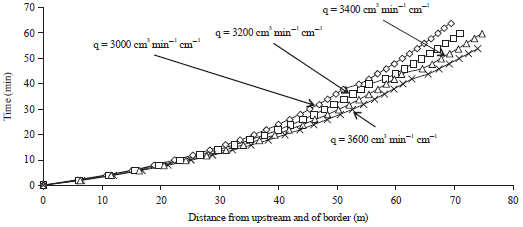 | |
| Fig. 1: | Water front advance curves for different stream sizes (q) |
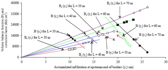 | |
| Fig. 2: | Determination of optimum values of (L) and (q) using volume balance function |
Considering y, yo and yd, respectively as accumulated total depth of water entering the soil at any point, total depth of water entering the soil at upstream end of border and design depth of application of water corresponding to an infiltration opportunity time of ’T’ for a border length ’L’, the first designcriteria needs to be satisfied is volume of water entered to the border till the advancing water front reaches the end must at least equal to volume required by the soil. This can be expressed as:
| (6) |
Further, a volume balance function (B), is derived expressing the difference between volume of water applied till the advancing water front reaches the end of the border and application of uniform depth (y0) of water over the entire border length1 as:
| (7) |
It is important to note that to allow for non-uniformities and non-parallel advance and recession curves, only values of ’B’ greater than some minimum values of ’Bd’ can accomplish adequate irrigation1, which can be expressed as:
| (8) |
where, f1 is a measure of excess water entered to the border.
Assuming border length selected for design trials as 30, 40, 50, 60 and 70 m, the values of T, yo, B and Bd for different border lengths and entrance stream sizes are estimated. The value of f1 is determined by experience and from the factors affecting the lack of parallelism of advance and recession curves16. To allow for non-parallelism of advance and recession curves, considering the factor of safety or a measure of the excess water (f1) as 0.216, the values of Bd are calculated for different border lengths and entrance stream sizes. Table 3 shows the values of T, yo, B and Bd for different border lengths and entrance stream sizes. Considering, B and Bd as ordinate against yo as abscissa with length of border (L) as parameters, a plot of B and Bd versus yo is obtained which is shown in Fig. 2. The intersection of B(yo) and Bd(yo) for a given length represents the minimum value of B which is acceptable for that length, since lower values would not provide adequate irrigation to all parts of the field. This point also represents the point of optimum application efficiency. In Fig. 2, the point of intersections of B(yo) and Bd(yo) for 30, 40, 50, 60 and 70 m lengths are shown.
| Table 3: | Values of T, yo, B and Bd for different trial border lengths and stream sizes |
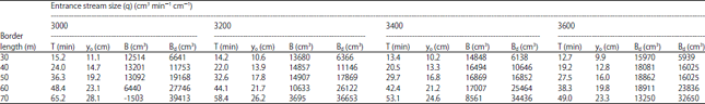 | |
T, yo, B and Bd, respectively represents infiltration opportunity time, total depth of water entering the soil at upstream end and volume balance function which is derived expressing the difference between volumes of water applied till the advancing water front reaches the end of the border and some minimum values of B that can accomplish adequate irrigation | |
From the Fig. 2, it is clear that if the design depth of application of each irrigation is 12.8 cm, the optimum border length is 30 m and if the depth of application is 15 cm, the optimum border length is 40 m and so on.
Considering the wheat crop on sandy loam soil under study, for which depth of water required to replenish the soil moisture in the root zone to field capacity is 15 cm, the optimum border length required is 40 m. Figure 3 clearly shows the intersection of B(yo) and Bd(yo) for 40 m length and the point of optimum application efficiency for wheat crop. Considering the optimum border length (L) as 40 m, design depth of application (yd) as 15 cm, time of application (T) as 24.78 minute and volume balance function (B) as 12000 cm3 (determined from Fig. 3), the optimum stream size is determined using Eq. 7, which equals to 2906 cm3 min–1 cm–1. The optimum border length and entrance stream size required to achieve maximum water application efficiency for crops other than wheat having different root zone depth, thus having different depth of water (yo) required to replenish the soil moisture in the root zone to field capacity, can be determined from the Fig. 2.
Application efficiency: The water application efficiency (Ea) is a measure of how efficiently the water is applied to the field. The definition of Ea has been fairly standardized25 as:
| (9) |
Using the notations as used in the text, volume of water added to the root zone and volume of water applied to the field corresponds to (yd L) and (qT), respectively. Hence Ea can be represented as:
![]()
Considering the derived values of yd, L, q and T as 15 cm, 40 m, 2906 cm3 min–1 cm–1, the water application efficiency equals 83.32%.
The results of this study give an application efficiency of the designed irrigation borders as 83.32%, which appears very significant as compared to the earlier studies carried out by different researchers26-29. Mangrio et al.26 studied the average water application efficiency under border irrigation method using different techniques and observed the average value as 67%. According to FAO27, the water application efficiency for border and furrow irrigation methods is up to 60%.
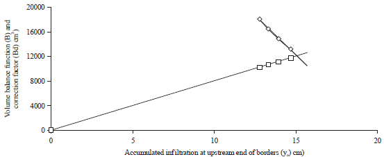 | |
| Fig. 3: | Determination of optimum value of (L) and (q) using volume balance function for wheat |
Figure shows the intersection of B (yo) and Bd (yo) for 40 m length and the point of optimum application efficiency for wheat crop. Considering the optimum border length (L) as 40 m, design depth of application (yd) as 15 cm, time of application (T) as 24.78 min and volume balance function (B) determined from graph as 12000 cm3, so that Eq. 9 can be applied to determine water application efficiency | |
The study carried out by Shaikh et al.28, in different areas reveals that application efficiencies for border irrigation method are within the ranges of 65-68% under medium textured soils. Further a study carried out on irrigation borders by Zerihun et al.29 achieved an application efficiency of 66.5%. In the above context, the maximum application efficiency that can be achieved is around 68% which is significantly low as compared to 83.32% achieved in the present study. Hence the present design methodology appears most appropriate in the of growing water needs of present days.
CONCLUSION
Following conclusions can be derived from the present study.
| • | The optimum border length and entrance stream size required to achieve maximum water application efficiency for wheat crop in sandy loam soil in the study area are 40 m and 2906 cm3 min–1 cm–1, respectively that gives application efficiency of 83.32% |
| • | The method is simple having easy field applicability as the plot of B and Bd versus yo, can be used to determine optimum border length and entrance stream size required to achieve maximum water application efficiency for various crops having different root zone depth |
| • | As prediction of water front advance-time relationship accurately and easily forms an important component in the efficient design of border irrigation system, use of modified technique to predict the water front advance-time relationship make the procedure simpler thus enhancing its field adaptability |
| • | The derived simplified method is also applicable to crops different from wheat and having different root zone depths |
SIGNIFICANCE STATEMENTS
This study discovers the methodology for the design of an irrigation border for all types of soils such that the water application efficiency becomes maximum. This study will be beneficial to researchers to design irrigation borders in the most efficient manner which many researchers were not able to explore.
REFERENCES
- Khanjani, M.J. and G.A. Barani, 1999. Optimum design of border irrigation system. J. Am. Water Resour. Assoc., 35: 787-792.
CrossRefDirect Link - Maheshwari, B.L. and T.A. McMahon, 1992. Modeling shallow overland flow in surface irrigation. J. Irrig. Drain. Eng., 118: 201-217.
CrossRefDirect Link - Alazba, A.A., 1997. Design procedure for border irrigation. Irrig. Sci., 18: 33-43.
CrossRefDirect Link - Davis, J.R., 1961. Estimating rate of advance for irrigation furrows. Trans. Am. Soc. Agric. Eng., 4: 52-54.
CrossRefDirect Link - Fok, Y.S. and A.A. Bishop, 1965. Analysis of water advance in surface irrigation. J. Irrig. Drain. Div., 91: 99-116.
Direct Link - Michael, A.M. and A.C. Pandya, 1971. Water front advance in irrigation borders. J. Agric. Eng. Res., 16: 62-71.
CrossRefDirect Link - Clemmens, A.J. and T. Strelkoff, 1979. Dimensionless advance for level-basin irrigation. J. Irrig. Drain. Divis., 105: 259-273.
Direct Link - Bishop, A.A., G.J. Poole, N.L. Allen and W.R. Walker, 1981. Furrow advance rates under surge flow systems. J. Irrig. Drain. Div., 107: 257-264.
Direct Link - Sherman, B. and V.P. Singh, 1982. A kinematic model for surface irrigation: An extension. Water Resour. Res., 18: 659-667.
CrossRefDirect Link - Singh, V. and S.M. Bhallamudi, 1996. Complete hydrodynamic border-strip irrigation model. J. Irrig. Drain. Eng., 122: 189-197.
CrossRefDirect Link - Walker, W.R. and G.V. Skogerboe, 1987. Surface Irrigation: Theory and Practice. Prentice-Hall, Hoboken, New Jersey, ISBN-13: 9780138779290, Pages: 386.
Direct Link - Clemmens, A.J., T. Strelkoff and A.R. Dedrick, 1981. Development of solutions for level-basin design. J. Irrig. Drain. Divis., 107: 265-279.
Direct Link - Parhi, P.K., 2016. An improvement to the waterfront advance-time relation for irrigation borders. Irrig. Drain., 65: 568-573.
CrossRefDirect Link - Smith, R.E., 1972. The infiltration envelope: Results from a theoretical infiltrometer. J. Hydrol., 17: 1-22.
CrossRefDirect Link - Parhi, P.K., S.K. Mishra and R. Singh, 2007. A modification to kostiakov and modified kostiakov infiltration models. Water Resour. Manage., 21: 1973-1989.
CrossRefDirect Link - Nash, J.E. and J.V. Sutcliffe, 1970. River flow forecasting through conceptual models part I-A discussion of principles. J. Hydrol., 10: 282-290.
CrossRefDirect Link - Mangrio, M.A., M.S. Mirjat, N. Leghari, N.H. Zardari and I.A. Shaikh, 2015. Evaluating water application efficiencies of surface irrigation methods at farmer's field. Pak. J. Agrc. Agric. Eng. Vet. Sci., 31: 279-288.
Direct Link - Shaikh, I.A., A. Wayayok, A.F.B. Abdullah, A.B.M. Soom and M. Mangrio, 2015. Assessment of water application losses through irrigation surveys: A case study of Mirpurkhas subdivision, Jamrao irrigation scheme, Sindh, Pakistan. Indian J. Sci. Technol., 8: 1-15.
Direct Link - Zerihun, D., C.A. Sanchez, K.L. Farrell-Poe and M. Yitayew, 2005. Analysis and design of border irrigation systems. Trans. ASAE, 48: 1751-1764.
CrossRefDirect Link