
Nabil Arman
Palestine Polytechnic University, Hebron, Palestine
Information Technology Journal
Year: 2005 | Volume: 4 | Issue: 4 | Page No.: 465-468


ABSTRACT
In this study, a comparison is conducted among three major representations of directed graphs to illustrate the main advantages and disadvantages of each representation scheme. In addition, a performance evaluation study is presented. The reason for conducting this study is to show that one of the schemes is overlooked despite the fact that it has more information than the other schemes and this information is very useful in improving the performance of many graph algorithms.
PDF Abstract XML References Citation
How to cite this article
Nabil Arman, 2005. Graph Representation: Comparative Study and Performance Evaluation. Information Technology Journal, 4: 465-468.
DOI: 10.3923/itj.2005.465.468
URL: https://scialert.net/abstract/?doi=itj.2005.465.468
DOI: 10.3923/itj.2005.465.468
URL: https://scialert.net/abstract/?doi=itj.2005.465.468
INTRODUCTION
Graph algorithms have attracted a large amount of research efforts due to the important role of these algorithms in many application domains. The efficiency of many graph algorithms is largely dependent on the underlying graph representation scheme. Many graph algorithms are well-documented in the literature, including specialized texts and research papers[1-5].
In this study, three directed graph representation schemes are compared, namely path matrix, adjacency matrix and adjacency lists.
GRAPH REPRESENTATION SCHEMES
The path matrix scheme is explained in detail, since it is not very popular compared to the other two schemes, which are well-known.
The path matrix graph representation: The path matrix is a special matrix/structure that has been used in answering the generalized forms of partially and fully instantiated same generation queries in deductive databases[1-3] and in computing the transitive closure of a database relation[5]. In this matrix, the rows represent some paths in the graph starting from the roots/source vertex to the leaves. Basically, depth-first search is used to create the paths of the graph. Instead of storing every vertex in all paths, the common parts of these paths can be stored only once to avoid duplications. If two paths P1 = <a1, a2,….., an, b1, b2,……., bm> and P2 = <a1, a2,….., an, c1, c2,……., cl> have the common parts <a1, a2,….., an> then P1 and P2 can be stored in the two consecutive rows of the matrix as <a1, a2,….., an, b1, b2,……., bm> and < -- n empty entries -- , c1, c2,……., cl>, where, the first n entries of the second row are empty.
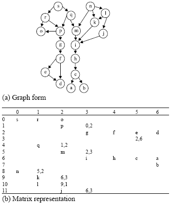 | |
| Fig. 1: | Directed graph in (a) Graph form (b) Matrix representation |
To prevent the duplicate storage of the vertex in the matrix, a different technique is used; for the first visit to the vertex, it is entered into the matrix and the coordinates of its location is recorded. On subsequent visits, instead of entering the vertex itself, its coordinates are entered into the matrix (a pointer to the already stored vertex). In this way, only a single copy of each of the graph’s vertex is guaranteed to be entered in the matrix. Moreover, there will be only one entry (either a vertex or a pointer) in the matrix for each edge in the graph. In Fig. 1b, the matrix representation of the graph given in Fig. 1a is presented.
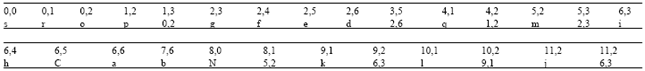 | |
| Fig. 2: | The matrix as linear array |
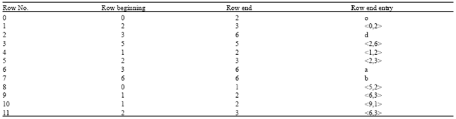 | |
| Fig. 3: | Matrix representation row beginnings and endings |
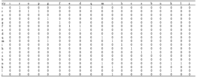 | |
| Fig. 4: | Adjacency matrix representation |
In that graph, there are 25 edges and in its matrix representation there are 25+2 =27 nonempty entries in the matrix (another two entries for the vertex s and n). An important advantage of this matrix structure is that it stores a path from each root to each vertex that is reachable from that root.
In the implementation of this sparse matrix, the empty entries are not stored explicitly. The matrix can be stored sequentially row by row as shown in Fig. 2. For each row, storing the column number, as shown in Fig. 3, of its first non-empty entry and the sequence of non-empty entries in the row is sufficient. Thus, the size of the stored matrix is much smaller than the original relation and matrix.
The adjacency matrix graph representation: The most straightforward scheme of directed graph representation is the so-called adjacency matrix representation. A V-by-V array of Boolean values is maintained, with a[x,y] set to true if there is an edge from vertex x to vertex y and false otherwise. The adjacency matrix representation for the graph in Fig. 1a is shown in Fig. 4. (1 means true and 0 means false). The first step in representing a graph is to map the vertex names to integers between 1 and V to make it possible to access information using array indexing[4].
The adjacency list graph representation: In this representation, all the vertices connected to each vertex
are listed on an adjacency list for that vertex. This can be easily done with linked lists. The linked lists are built as usual, with artificial nodes for the beginning of the lists kept in an array adj indexed by vertex. To add an a directed edge connecting x to y to this representation of the graph, we add y to x’s adjacency list[4].
COMPARISON CRITERIA
The three representation schemes are compared according to the following criteria:
Intelligence and pruning: Algorithms that use the path matrix representation can benefit from the properties of this representation to prune or bound the traversing of the vertices in the matrix, since it terminates the search once a pointer goes beyond the vertex that the algorithm tries to reach and then backtracks from there. On the other hand, algorithms that use the adjacency matrix or adjacency list representations may explore irrelevant parts of the graph. Assume we are trying to determine whether there is a path from vertex v1 to vertex v2 (a query that might be called a path existence query). If DFS starts with v1, then it will consider all vertices reachable from that vertex until it reaches v2 (if v2 is reachable). However, if DFS starts with v1 and uses the path matrix representation, then it will consider vertices reachable from that vertex as long as no vertex coordinates goes beyond the coordinates of vertex v2 or until it reaches v2 (if v2 is reachable).
Database usage (vertex clustering): An important advantage of the path matrix representation is that it stores a path from the source vertices to all vertices reachable from that source vertex. Clustering vertices around source vertices reduces the number of page I/Os necessary to process data needed in many graph algorithms. On the other hand, the way adjacency matrix representation keeps its information increases dramatically the number of page I/Os necessary to process data in graph algorithms.
Path ordering: In the path matrix representation, paths have implicit order according to the rows they appear in. On the other hand, neither adjacency matrices nor adjacency lists have such order. This ordering plays a crucial role in pruning the search of graphs once a certain path number has been exceeded.
Space requirements: As explained before, in the implementation of the path matrix representation, the empty entries are not stored explicitly. The matrix can be stored sequentially row by row as shown in Fig. 2. For each row, storing the column number, as shown in Fig. 3, of its first non-empty entry and the sequence of non-empty entries in the row is sufficient. Thus, the size of the stored matrix is much smaller than the original graph and matrix. The space requirement is actually proportional to |E|+|s| where, |E| is the number of edges and |s| is the number of source nodes (|s| is generally a constant).
However, the adjacency matrix representation needs space proportional to |V|2 and the adjacency list representation needs space proportional to |V|+|E|. Therefore, the space needed by path matrix representation is less than the space needed by the other two representation schemes.
Vertex skipping in searching: In certain path algorithms, such as finding the path length between two vertices, or finding the maximum/minimum path length between two vertices, or even checking the path existence between two vertices, path matrix representation enables these algorithms to skip many vertices on different paths, instead of considering all vertices on these paths, using the row beginnings and row ends to determine the paths or path lengths.
PERFORMANCE EVALUATION
To determine the performance of graph algorithms that use the three representation schemes, simulations were performed for random graphs with 2000 edges of 4 different out degree values from 1 to 4 as shown in Fig. 5. For more accurate results, the algorithms were executed 5 times for each case and the average was taken (Fig. 5). The path existence query was chosen as representative of graph algorithms and was tested for 100 randomly generated queries. The number of nodes visited to answer these queries was determined for the three representation schemes. When the graph obtained from the execution of the algorithms was examined, two things were observed.
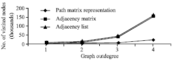 | |
| Fig. 5: | Comparative performance for the path existence query of different graph representation schemes |
First, the number of nodes visited in the algorithm that uses the path matrix representation (where the row beginnings and row ends of the matrix representation are visited only) is less than the number of nodes visited in the other two schemes of graph representation (where all nodes along the paths are visited). Second, increasing the outdegree of the underlying graph is in favor of the path matrix representation scheme. This is due to the fact that larger outdegree values of the underlying graph generate longer paths of the graph, which results in skipping larger number of nodes in the graph.
CONCLUSIONS
This study presents a comparative study and performance evaluation of algorithms that use different graph representation schemes. Each representation scheme is explained briefly and its main advantages and disadvantages is presented. The criteria are useful in choosing the appropriate representation scheme for different internal or external algorithms. The study also highlights the advantages of path matrix representation scheme since it is overlooked in graph theory related algorithms.
REFERENCES
- Arman, N., 2005. Graph representation comparative study. Proceedings of the International Conference on Foundations of Computer Science, June 27-30, 2005, Las Vegas, USA., pp: 1-5.
Direct Link