
Tzong-Mou Wu
Department of Mechanical Engineering, Far East College, Tainan 744, Taiwan
Journal of Applied Sciences
Year: 2004 | Volume: 4 | Issue: 3 | Page No.: 398-405


ABSTRACT
In general, the kinematics design problems include two types: synthesis of mechanism and inverse of robot. In fact, when we deal with the design problems, the results/outputs usually are given/desired but the inputs are unknown/to be found. People must understand how to control/determine the input variables to satisfy the results/outputs. This paper systematically presents these two types of solution based on transformation matrix and Homotopy continuation method for general kinematics design problems except for mechanism and robot. The kinematic equations, which include displacement, velocity and acceleration relationships, are derived by 4x4 homogeneous transformation matrix method. Also these equations can be solved by Homotopy continuation method when these equations are non-linear.
PDF Abstract XML References Citation
How to cite this article
Tzong-Mou Wu, 2004. The Kinematics Design Problems. Journal of Applied Sciences, 4: 398-405.
DOI: 10.3923/jas.2004.398.405
URL: https://scialert.net/abstract/?doi=jas.2004.398.405
DOI: 10.3923/jas.2004.398.405
URL: https://scialert.net/abstract/?doi=jas.2004.398.405
INTRODUCTION
Although the analysis methods of kinematics have been carried out step by step far from the 17th century, such as the geometrical method, vector analysis, principle of work and energy, etc., are the well-known and popular kinematics analysis methods[1,2]. They are forward analysis problems. Nevertheless, in some real backward problems, the outputs usually are given/desired and the inputs are to be found/unknown. The studies of mechanisms and robots, are branches of kinematics, have considered this problem[3-6]. However, the traditional courses of kinematics do not consider design problems. They are all the problems of analysis.
In the process of solving kinematics design problems, some troublesome simultaneous equations would be generated, especially the simultaneous non-linear equations. Up to the present, we have already many different methods can manage the simultaneous non-linear equations, such as Newton-Raphson method[7]. But the solutions can not be guaranteed by these typical numerical techniques. This paper attempt to use Homotopy continuation method[8,9,14] to solve the simultaneous non-linear equations because of the convergence speed of continuation method is faster and we also can guarantee the solutions by this method. Furthermore, the 4x4 homogeneous transformation matrices are applied to systematically derive the kinematic displacement, velocity and acceleration equations[13].
With the computer improved and the numerical continuation technique developed, the solutions of design variables in kinematics design problems are not difficult. We can use current high-speed processor to determine the solutions quickly. Also, we almost can real-time control the necessary inputs to meet the specified outputs whatever displacement, velocity or the acceleration. An example is given in this paper to explain the overall procedure of solving kinematics design problems.
The kinematics design problems: The objects of kinematics studies are to obtain the “equations of motion” or “kinematic equations”, i.e. the displacement, velocity and acceleration relationships between input variables and output variables. These equations can be derived by serial combination of 4x4 homogeneous transformation matrices. As we known, the nominal position and orientation of the kth frame (XYZ)k with respect to the base frame (XYZ)0 can be written as
| (1) |
Where Ai is the basic rotational or translational matrix i-1Ai and they have four standard 4x4 homogeneous forms
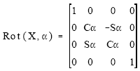 |
 |
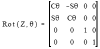 | (2) |
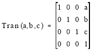 |
Where Rot, Tran, C and S mean the rotation, translation, cos and sin, respectively. For the general k linkages, the displacement equation is
| (3) |
Where kr is the displacement or position vector of analyzed point with respect to frame (XYZ)k. After the displacement relationship of kinematic equations being determined from equation (3), we then differentiate it two times to get velocity and acceleration relationships, respectively.
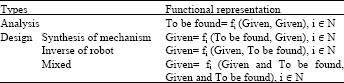
Whatever how complicated these three kinematic equations are. All the kinematic equations have two types: forward/analysis and backward/design and can be represented by the following general functional forms
| (4) |
The givens and unknowns in forward/analysis and backward/design questions are usually reverse. Generally, in the analysis problems, the givens are all the input variables, including fixed and changeable variables and the unknowns are the output variables. However, we have two kinds of design problems in equations (4). One is to find input fixed variables but outputs and input changeable variables are given, e.g. the synthesis of mechanism. Another is to find input changeable variables but outputs and input fixed variables are known, for example, the inverse of robot manipulator. Sometimes, the design problems could not be completely classified according to these two types. Since we perhaps have the geometrical constraints in the equations of motion. Therefore, some of the input fixed or changeable variables also maybe are the unknowns. Anyway, the outputs must be given in general so-called design problems. Now, we rewrite equations (4) by the four types (Table 1).
| Table 1: | The types and functional representation of analysis and design |
 | |
To solve equations (4) regardless of they are what type in Table 1, we always have two kinds, i.e., linear and non-linear. We can use Gauss elimination to easily solve the simultaneous linear equations. However, for high order, hyper or non-linear equations, we must by the help of special simplification artifice or numerical techniques.
When dealing with the numerical problem, such as the Newton-Raphson method, there are two troublesome questions. One is the good initial guesses are not easy to detect and another is we worry whether the method we use will converge into useful solutions. Continuation method can eliminate these shortcomings.
Given a set of equations in n variables x1, x2, … , xn. We modify the equations by omitting some of the terms and adding new ones until we have a new system of equations, the solutions to which may be easily guessed/given/known. We then deform the coefficients of the new system into the coefficients of the original system by a series of small increments and we follow the solution through the deformation, using methods such as Newton-Raphson. This is called Homotopy continuation original system.
If we wish to find the solution vector for a system of simultaneous equations written in the form:
| (5) |
We choose a new simple start system:
| (6) |
That must be known or controllable and easy to solve. Then, we define the Homotopy continuation function as:
| (7) |
Where t is an arbitrary parameter and varies from 0 to 1, i.e., t ∈ [0, 1]. Therefore, we have the following two boundary conditions
| (8) |
This is called Homotopy continuation method. It is also called Bootstrap method or Parameter-Perturbation method, but these names did not become popular.
In the following section, we will present the different approaches and show the overall procedure of solving kinematics design problems.
Example: At the instant shown in Fig. 1, the tractor is traveling forward with a displacement, velocity and acceleration of a m/s, ![]() m/s and ä m/s2. The pilot is rotating about the Z axis, exactly Z1 axis in Fig. 2, with an angle θ rad, an angular velocity
m/s and ä m/s2. The pilot is rotating about the Z axis, exactly Z1 axis in Fig. 2, with an angle θ rad, an angular velocity ![]() rad/s and an angular acceleration
rad/s and an angular acceleration ![]() rad/s2. At this same instant, the arm ABC is rotating with φ rad,
rad/s2. At this same instant, the arm ABC is rotating with φ rad, ![]() rad/s and
rad/s and ![]() rad/s2 those measured relative to the tractor frame (XYZ)1. l1 and l2 are the structure dimensions of the tractor. The arm ABC is a robot manipulator. Although it is not this paper’s study, the coordinates of its ending point P w.r.t. (XYZ)2 still can be represented as vector 2r = [2Px, 2Py, 2Pz, 1]T. In this paper, we will synthesize l1, l2 and invert outputs 0r, 2r to determine inputs
rad/s2 those measured relative to the tractor frame (XYZ)1. l1 and l2 are the structure dimensions of the tractor. The arm ABC is a robot manipulator. Although it is not this paper’s study, the coordinates of its ending point P w.r.t. (XYZ)2 still can be represented as vector 2r = [2Px, 2Py, 2Pz, 1]T. In this paper, we will synthesize l1, l2 and invert outputs 0r, 2r to determine inputs ![]() .
.
Before we proceed these two kinematics design problems, we have to derive the equations of motion. Firstly, we redraw the real façade Fig. 1 as the dimensional profile Fig. 2. Therefore, the coordinate transformation relationships are:
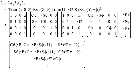 | (9) |
Then, we differentiate above equation by time to yield
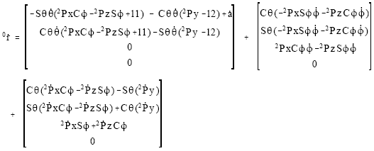 | (10) |
Similarly,
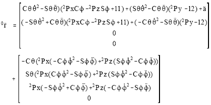 |
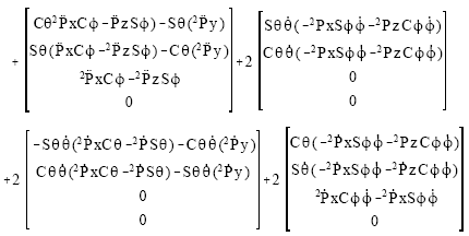 | (11) |
Case 1: The synthesis of structure dimensions l1 and l2
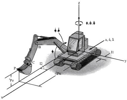 | |
| Fig. 1: | The real façade of the tractor and its corresponding assignments |
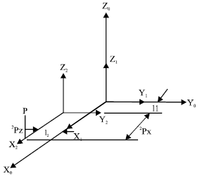 | |
| Fig. 2: | The dimensional profile of the tractor and its coordinate system |
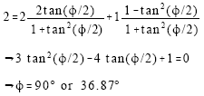
Observing equation (9), we have four sets of variables (l1, l2), (a, θ, φ), 0r and 2r as well as three equations. To determine (l1, l2), we need to assign our desired outputs 0r = [3, -1, 2, 1]T, 2r = [2, 0, 1, 1]T and partial input variables (a, θ, φ) = (0, 300, 300). However, we just have two independent equations in equation (9), i.e., first and second row equations. Since the variables in third row equation are not unknown. It is very easy to contradict for the solution in this equation if we give 0Pz, 2Px, 2Pz and φ angle together. So we must free one variable to satisfy this equation. According to our previous section explanation “the outputs must be given in general so-called design problems”, hence we decide free φ angle to be unknown. This equation therefore becomes mixed type of design in Table 1 and has following form:
| (12) |
We must firstly apply trigonometric formulas to solve this equation exactly, then this case will be real synthesis problem, i.e. outputs and input changeable variables are given just input fixed variables are to be found, as follows
 | (13) |
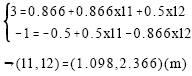
We substitute 0r = [3, -1, 2, 1]T, 2r = [2, 0, 1, 1]T and (a, θ, φ) = (0, 300, 900) into equation (9). This equation is a set of simultaneous linear equations and the synthesis answer is very easy to be obtained
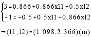 | (14) |
| 20 For φ = 36.870 |
We substitute 0r = [3, -1, 2, 1]T, 2r = [2, 0, 1, 1]T and (a, θ, φ) = (0, 300, 36.870) into equation (9). Similarly,
 | (15) |
Case 2: The inverse of outputs 0r, 2r and inputs
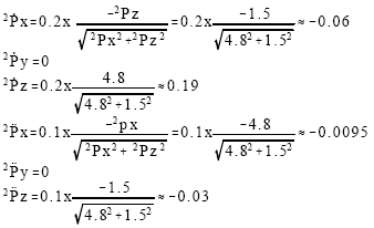
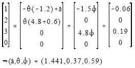
In the same way, from equation (9), we have four sets of variables (l1, l2), (a, θ, φ), 0r and 2r as well as three equations. To determine (a, θ, φ), we need to assign our desired outputs 0r = [5.4, -1.2, 1.5, 1]T, 2r = [4.8, 0, 1.5, 1]T where (l1, l2) = (0.6, 1.2)[13]. Substituting these givens into equation (9) to yield
 | (16) |
Clearly, this equation is a set of simultaneous non-linear equations. Its solutions would be found by Homotopy continuation method. If we let
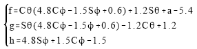 | (17) |
And the start equations are
 | (18) |
Where
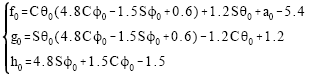 | (19) |
Now, we define the Homotopy equations as
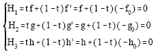 | (20) |
 | |
| Fig. 3: | Specified motion of the ending point P of the tractor measured by (XYZ)2 |
 | |
| Fig. 4: | The numerical results of Homotopy continuation method in case 2 |
| Appendix: |
 |
 |
Solve above simultaneous equations by changing t from 0 to 1, see appendix for programming and Fig. 4 for the numerical results of Homotopy continuation method. The program takes us just only about 1.44 second to run this example in merely AMD-K6/2-500 CPU. We obtain the convergence answers from above simultaneous equations
| (21) |
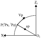
Consider Fig. 3, if we pay attention to a circular motion with a constant tangential speed vp = 0.2 m s-1 and acceleration ap = 0.1 m s-2 focuses on the circular center O2, these are all measured by coordinate (XYZ)2. From this figure, we compute the following component information
 | (22) |
Assuming that our desired velocity and acceleration outputs at ending point P of the tractor measured by base frame (XYZ)0, respectively are
| (23) |
Substituting these data into equation (10), we obtain the following simultaneous linear equations and the answers
 | (24) |
In like manner, from equation (11), we have
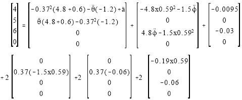 | (25) |
Finally, the necessary accelerations therefore are
| (26) |
Kinematics is a branch of physics. Many words were devoted to the studies of kinematics far from the 17th century. The geometrical method, vector analysis, principle of work and energy and so on, were the well-known and popular kinematics analysis methods. However, these studies seem to interest in the forward analysis kinematics problems. Traditionally, the backward design kinematics problems were not yet completely discussed except for the fields of mechanisms and robots.
Typically, it is usually a big trouble and disadvantage for us to do the algebraic operation, for example, solving the non-linear equations. Fortunately, by the aid of computer science, the non-linear equations will be solved no more difficulty. We have many different numerical methods can help us to treat these equations. Homotopy continuation is one of the famous methods. Its convergence speed is faster, also the algorithm is clear and easy. This paper applies this method to solve the simultaneous non-linear equations.
Moreover, in analyzing the kinematics problems, we usually need the “kinematic equations” and some mathematical operations such as calculus, inner or cross product, etc. So we have to more carefully consider the required mathematical operations. With the method of vector analysis, we must firstly determine the angular velocity and angular acceleration to find the linear velocity and acceleration. It is not convenient for us to analyze the kinematics problems. This paper presents systematic 4x4 homogeneous transformation matrices to overcome this imperfection. By means of matrices operation, we can easier to obtain the kinematic equations than traditional vector analysis method. These interesting methods will provide other analysis and design approaches. It is hoped that the work presented here will contribute towards progress in the kinematics analysis and design techniques and other scientific fields for scientists and engineers.