
S.B. Imandoust
Department of Economic, Payame Noor University, Mashhad, Iran
S.M. Fahimifard
Department of Agricultural Economics Engineering, University of Zabol, Zabol, Iran
Journal of Applied Sciences
Year: 2010 | Volume: 10 | Issue: 13 | Page No.: 1263-1270


ABSTRACT
The aim of this research is studying the application of NNARX as a nonlinear dynamic neural network model in contrast with ARIMA as a linear model to forecast Iran’s agricultural economic variables. As a case study the three horizons (1, 2 and 4 week ahead) of Iran’s rice, poultry and egg retail price are forecasted using the two mentioned models. The results of using the three forecast evaluation criteria (R2, MAD and RMSE) state that, NNARX model outperforms ARIMA model in agricultural economic variables forecasting.
PDF Abstract XML References Citation
Received: March 16, 2010;
Accepted: May 04, 2010;
Published: June 10, 2010
How to cite this article
S.B. Imandoust and S.M. Fahimifard, 2010. Application of NNARX to Agricultural Economic Variables Forecasting. Journal of Applied Sciences, 10: 1263-1270.
DOI: 10.3923/jas.2010.1263.1270
URL: https://scialert.net/abstract/?doi=jas.2010.1263.1270
DOI: 10.3923/jas.2010.1263.1270
URL: https://scialert.net/abstract/?doi=jas.2010.1263.1270
INTRODUCTION
In the last few decades, many forecasting models have been developed (Makridakis, 1982). Which among them, the Auto-Regressive Integrated Moving Average (ARIMA) model has been highly popularized, widely used and successfully applied not only in economic time series forecasting, but also as a promising tool for modeling the empirical dependencies between successive times and failures (Ho and Xie, 1998). Recently, it is well documented that many economic time series observations are non-linear while, a linear correlation structure is assumed among the time series values therefore, the ARIMA model can not capture nonlinear patterns and, approximation of linear models to complex real-world problem is not always satisfactory. While nonparametric nonlinear models estimated by various methods such as Artificial Intelligence (AI), can fit a data base much better than linear models and it has been observed that linear models, often forecast poorly which limits their appeal in applied setting (Racine, 2001).
Artificial Intelligence (AI) systems are widely accepted as a technology offering an alternative way to tackle complex and ill-defined problems (Kalogirou, 2003). They can learn from examples, are fault tolerant in the sense that they are able to handle noisy and incomplete data, are able to deal with non-linear problems and once trained can perform prediction and generalization at high speed (Kamwa et al., 1996). They have been used in diverse applications in control, robotics, pattern recognition, forecasting, medicine, power systems, manufacturing, optimization, signal processing and social/psychological sciences. AI systems comprise areas like expert systems, Artificial Neural Network (ANN), genetic algorithms, fuzzy logic and various hybrid systems, which combine two or more techniques (Kamwa et al., 1996). Among the mentioned AI systems, according to Haykin, a neural network is a massively parallel-distributed processor that has a natural propensity for storing experiential knowledge and making it available for use (Haykin, 1994). Also, the greatest advantage of a neural network is its ability to model complex nonlinear relationship without a priori assumptions of the nature of the relationship like a black box (Karayiannis and Venetsanopoulos, 1993).
In dynamic networks (such as Neural Network Auto-Regressive model with eXogenous inputs (NNARX), the output depends not only on the current input to the network, but also on the current or previous inputs, outputs, or states of the network. Dynamic networks are generally more powerful than static networks (although somewhat more difficult to train). Because dynamic networks have memory, they can be trained to learn sequential or time-varying patterns (Racine, 2001).
Concerning the application of neural nets to time series forecasting, there have been mixed reviews. For instance, Laepes and Farben (1987) reported that simple neural networks can outperform conventional methods, sometimes by orders of magnitude. Sharda and Patil (1990) conducted a forecasting competition between neural network models and traditional forecasting technique (namely the Box-Jenkins method) using 75 time series of various natures. They concluded that simple neural nets could forecast about as well as the Box-Jenkins forecasting system. Wu (1995) conducts a comparative study between neural networks and ARIMA models in forecasting the Taiwan/US dollar exchange rate. His findings show that neural networks produce significantly better results than the best ARIMA models in both one-step-ahead and six-step-ahead forecasting. Similarly, Hann and Steurer (1996), Zhang and Hu (1998) find results in favor of neural network. Gencay (1999) compares the performance of neural network with those of random walk and Generalized Auto-Regressive Conditional Hetroskedastic (GARCH) models in forecasting daily spot exchange rates for the British pound, Deutsche mark, French franc, Japanese yen and the Swiss franc. He finds that forecasts generated by neural network are superior to those of random walk and GARCH models. Ince and Trafalis (2006) proposed a two stages forecasting model which incorporates parametric techniques such as Auto-Regressive Integrated Moving Average (ARIMA), Vector Auto-Regressive (VAR) and co-integration techniques and nonparametric techniques such as Support Vector Regression (SVR) and Artificial Neural Networks (ANN) for exchange rate prediction. Comparison of these models showed that input selection is very important. Furthermore, findings showed that the SVR outperforms the ANN for two input selection methods. Haoffi et al. (2007) introduced a Multi-Stage Optimization Approach (MSOA) used in back-propagation algorithm for training neural network to forecast the Chinese food grain price. Their empirical results showed that MSOA overcomes the weakness of conventional BP algorithm to some extend. Furthermore, the neural network based on MSOA can improve the forecasting performance significantly in terms of the error and directional evaluation measurements. Fahimifard (2008) compared the Adaptive Neuro Fuzzy Inference System (ANFIS) and ANN as the nonlinear models with the ARIMA and GARCH as the linear models to Iran’s meat, rice, poultry and egg retail price forecasting. His research stated that nonlinear models overcome the linear models strongly.
Fahimifard et al. (2009) studied the application of ANFIS in Iran’s poultry retail price forecasting in contrast with ARIMA model. Their findings stated that ANFIS outperforms the ARIMA model in all three 1, 2 and 4 weeks ahead.
In this study, the application of NNARX as a nonlinear dynamic neural network model will compare with the ARIMA as a linear model. In order to comparison of mentioned models the common forecast performance measures such as absolute fraction of variance (R2), Mean Absolute Deviation (MAD) and Root Mean Square Error (RMSE) are used. As an empirical application, the various forecasting performance of mentioned models for three perspectives (1, 2 and 4 week ahead) of Iran’s rice, poultry and egg retail price weekly time series are compared via common forecast performance measures.
MATERIALS AND METHODS
Auto-Regressive Integrated Moving Average (ARIMA) model: Introduced by Box and Jenkins (1970), in the last few decades the ARIMA model has been one of the most popular approaches of linear time series forecasting methods. An ARIMA process is a mathematical model used for forecasting. One of the attractive features of the Box-Jenkins approach to forecasting is that ARIMA processes are a very rich class of possible models and it is usually possible to find a process which provides an adequate description to the data. The original Box-Jenkins modeling procedure involved an iterative three-stage process of model selection, parameter estimation and model checking. Recent explanations of the process (Makridakis et al., 1998) often add a preliminary stage of data preparation and a final stage of model application (or forecasting).
Also, the ARIMA (p, d, q) model for variable x is as follow:
| (1) |
where, y is estimated by the following equation:
| (2) |
where, yt and et are the target value and random error at time t, respectively, φi = (i = 1, 2,...p) and θj = (j = 1, 2,...q) are model parameters, p and q are integers and often referred to as orders of autoregressive and moving average polynomials and L and d refer to lag number an orders of integration.
Neural Network Auto-Regressive model with eXogenous (NNARX) inputs: Neural networks can be classified into dynamic (e.g., NNARX) and static (e.g., ANN) categories. Static networks have no feedback elements and contain no delays; the output is calculated directly from the input through feed-forward connections. In dynamic networks, the output depends not only on the current input to the network, but also on the current or previous inputs, outputs, or states of the network. Dynamic networks are generally more powerful than static networks (although somewhat more difficult to train). Because dynamic networks have memory, they can be trained to learn sequential or time-varying patterns (Medsker and Jain, 2000). This model has a parametric component plus a nonlinear part, where the nonlinear part is approximated by a single hidden layer feed-forward ANN. The Neural Network Auto-Regressive with Exogenous (NNARX) inputs is current dynamic network, with feedback connections enclosing several layers of the network. The NNARX model is based on the linear ARX model, which is commonly used in time-series modeling. Also, this has applications in such disparate areas as prediction in financial markets (Roman and Jameel, 1996), channel equalization in communication systems (Feng et al., 2003), phase detection in power systems (Kamwa et al., 1996), sorting (Jayadeva and Rahman, 2004), fault detection (Chengyu and Danai, 1999), speech recognition (Robinson, 1994) and even the prediction of protein structure in genetics (Pollastri et al., 2002).
The defining equation for the NNARX model is as follow:
| (3) |
where, the next value of the dependent output signal y(t) is regressed on previous values of the output signal and previous values of an independent (exogenous) input signal. The output is feed back to the input of the feed-forward neural network as part of the standard NNARX architecture, as shown in the Fig. 1a. Because the true output is available during the training of the network, a series-parallel architecture can be created (Rosenblatt, 1961), in which the true output is used instead of feeding back the estimated output, as shown in the Fig. 1b. This has two advantages. The first is that the input to the feed-forward network is more accurate. The second is that the resulting network has purely feed-forward architecture and static backpropagation can be used for training.
Dynamic networks are trained in the same gradient-based algorithms that were used in backpropagation. Although they can be trained using the same gradient-based algorithms that are used for static networks, the performance of the algorithms on dynamic networks can be quite different and the gradient must be computed in a more complex way (De Jesus and Hagan, 2001a). A diagram of the resulting network is shown by Fig. 2, where a two-layer feed-forward network is used for the approximation:
Each layer is made up of the following parts:
| • | Set of weight matrices that come into that layer (which can connect from other layers or from external inputs), associated weight function rule used to combine the weight matrix with its input (normally standard matrix multiplication, dotprod) and associated tapped delay line |
| • | Bias vector |
| • | Net input function rule that is used to combine the outputs of the various weight functions with the bias to produce the net input (normally a summing junction, netprod) |
| • | Transfer function |
 | |
| Fig. 1: | (a) Parallel and (b) series-parallel architectures |
 | |
| Fig. 2: | A typical Neural Network Auto-Regressive with Exogenous (NNARX) inputs |
The network has inputs that are connected to special weights, called input weights and denoted by IWi,j (net.IW{i, j} in the code), where j denotes the number of the input vector that enters the weight and i denotes the number of the layer to which the weight is connected. The weights connecting one layer to another are called layer weights and are denoted by LWi, j (net.LW{i, j} in the code), where j denotes the number of the layer coming into the weight and I denotes the number of the layer at the output of the weight. This type of network's weights has two different effects on the network output. The first is the direct effect, because a change in the weight causes an immediate change in the output at the current time step (This first effect can be computed using standard backpropagation). The second is an indirect effect, because some of the inputs to the layer, such as a(t, 1), are also functions of the weights. To account for this indirect effect, the dynamic backpropagation must used to compute the gradients, which are more computationally intensive (De Jesus and Hagan, 2001a). Expect dynamic backpropagation to take more time to train, in part for this reason. In addition, the error surfaces for dynamic networks can be more complex than those for static networks. Training is more likely to be trapped in local minima. This suggests that you might need to train the network several times to achieve an optimal result (De Jesus and Hagan, 2001b).
DATA DESCRIPTION
For the exercise which is follows, the Iran’s agricultural products retail price is modeled as a function of past prices. Clearly, this has the shortcoming that our models are somewhat naive from the perspective of theoretical macroeconomics. However, there is a large body of literature in economics suggesting that very parsimonious models, such ARIMA model, perform better than more complex models, at least from the perspective of forecasting (Chen et al., 2001). The research was conducted from 2009:02 to 2010:02. The weekly Iran’s agricultural products retail price time series for the period 2002:03-2008:06 has been obtained from the website of Iran State Livestock Affairs Logistics (www.IranSLAL.com). Also, the periods 2002:03-2006:07 (70% of total observations) and 2006:07-2008-06 (30% of total observations) are considered for training and testing of all models, respectively.
FORECAST PERFORMANCE MEASURES
According to Table 1 beside, forecast researchers need measures in order to compare the forecasting performance of various models. Commonly, these measures are including of R2, MAD and RMSE that the following is their definition and general formulas:
RESULTS AND DISCUSSION
ARIMA performance to agricultural products retail price forecasting: For ARIMA model the degree of integration (d), autoregressive (p) and moving average (q) have been identified by Dikes-Fuller, correlation and partial correlation diagrams, respectively. The Schwartz-Bayesian criterion has been used for identification of lag number.
| Table 1: | Three common types of forecast performance measures |
 | |
The forecasting performance of Iran’s rice, poultry and egg retail price obtained by the ARIMA model has been shown in Fig. 3.
Figure 3 demonstrates the out-sample fitness of the best designed structures of ARIMA models for forecasting 1, 2 and 4 weeks ahead of Iran’s rice, poultry and egg retail price in comparison with the actual observations. And Fig. 3 presents the values of evaluation criterions correspond to the best ARIM structure for forecasting the considered horizons. According to the above table the accuracy of Iran’s rice, poultry and egg retail price forecasting used ARIMA model will reduced during the time horizon increscent because of the higher RMSE and MAD and lower R2.
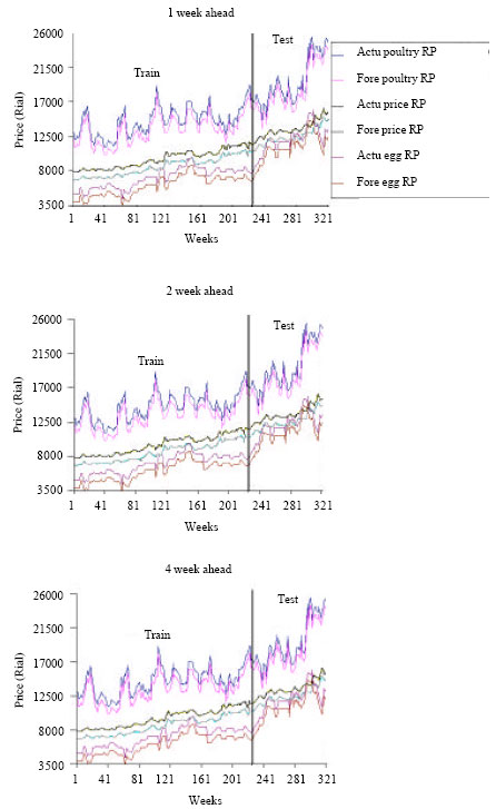
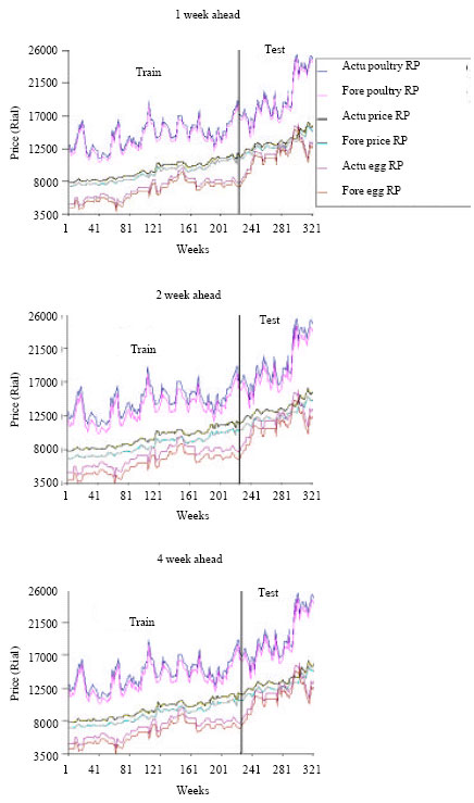
NNARX performance to agricultural products retail price forecasting: For non-linear part of NNARX the various architectures of feed-forward backpropagation network have been investigated. The forecasting performance of Iran’s rice, poultry and egg retail price obtained by the NNARX model has been shown in Fig. 4.
Similarly, the Fig. 4 demonstrates the train and test fitness of the best designed structures of NNARX models for forecasting 1, 2 and 4 weeks ahead of Iran’s rice, poultry and egg retail price in comparison with the actual observations. And Fig. 4 presents the values of evaluation criterions correspond to the best NNARX structure for forecasting the considered horizons. Similarly, According to the Fig. 4 the accuracy of Iran’s rice, poultry and egg retail price forecasting used NNARX model will reduced during the time horizon increscent because of the higher RMSE and MAD and lower R2.
Figure 3 and 4 show that NNARX model provides the better forecasting results for Iran’s rice, poultry and egg retail price forecasting by all three performance measures, because of the highest values of R2, lowest values of MAD and RMSE criteria in comparison with the ARIMA model.
 | |
 | |
| Source: Research findings | |
| Fig. 3: | Forecast performance of Iran’s agricultural products price used ARIMA model |
 | |
 | |
| Fig. 4: | Forecast performance of Iran’s agricultural products price used NNARX model |
| Table 2: | Comparision of NNARX and ARIMA models for forecasting |
 | |
Comparison of NNARX and ARIMA models to agricultural products retail price forecasting: In order to compare the performance of considered linear and nonlinear models to Iran’s rice, poultry and egg retail price forecasting, we divided the values of forecast evaluation criterions of NNARX to ARIMA model per each horizon, Table 2 demonstrates the results of these comparisons.
According to the Table 2, the NNARX nonlinear model forecasting performance is better in contrast with the ARIMA linear model because (1) the RMSE and MAD divided are less than 1 and 2 the R2 divided is more than 1.
CONCLUSION
Non-linear processes are usually too complicated for accurate modeling by traditional and statistical models, therefore there are always rooms for alternative model types such as the data based models. Clearly, more research is needed to see if and how the proposed scheme could help the development of efficient models.
In this study, the application of NNARX as a nonlinear dynamic neural network model and ARIMA as a linear model compared for agricultural economic variables forecasting. As an empirical application, the various forecasting performance of mentioned models for three perspectives (1, 2 and 4 week ahead) of Iran’s rice, poultry and egg retail price weekly time series were compared via common forecast performance measures. Results indicated that NNARX nonlinear model forecasts are considerably more accurate than the linear traditional ARIMA model which used as benchmarks in terms of error measures, such as RMSE and MAD. On the other hand, as the R2 criterion is concerned; NNARX nonlinear model is absolutely better than ARIMA linear model. Briefly using forecast evaluation criteria has been demonstrated that NNARX nonlinear model outperforms ARIMA model.
REFERENCES
- Chen, X., J. Racine and R.N. Swanson, 2001. Semiparametric ARX neural network models with an application to forecasting inflation. IEEE Trans. Neural Networks, 12: 674-683.
CrossRefDirect Link - Chengyu, G. and K. Danai, 1999. Fault diagnosis of the IFAC benchmark problem with a model-based recurrent neural network. Proceedings of the 1999 IEEE International Conference on Control Applications, Aug. 22-27, IEEE Computer Society, Los Alamitos, CA, USA., pp: 1755-1760.
CrossRef - De Jes�s, O. and M.T. Hagan, 2001. Backpropagation through time for a general class of recurrent network. Proceedings of the International Joint Conference on Neural Networks, July 15�19, Washington, DC, USA., pp: 2638-2642.
CrossRef - De Jesus, O. and M.T. Hagan, 2001. Forward perturbation algorithm for a general class of recurrent network. Proceedings of the International Joint Conference on Neural Networks, July 15�19, Washington, DC, USA., pp: 2626-2631.
CrossRef - Fahimifard, S.M., M. Salarpour, M. Sabouhi and S. Shirzady, 2009. Application of ANFIS to agricultural economic variables forecasting case study: Poultry retail price. Int. Artif. Intell., 2: 65-72.
CrossRefDirect Link - Feng, J., C.K. Tse and F.C.M. Lau, 2003. A neural-network-based channel-equalization strategy for chaos-based communication systems. IEEE Trans. Circ. Syst. Fund. Theor. Appl., 50: 954-957.
CrossRef - Gencay, R., 1999. Linear, non-linear and essential foreign exchange rate prediction with simple technical trading rules. J. Int. Econ., 47: 91-107.
CrossRef - Pollastri, G., D. Przybylski, B. Rost and P. Baldi, 2002. Improving the prediction of protein secondary structure in three and eight classes using recurrent neural networks and profiles. Proteins, 47: 228-235.
PubMed - Hann, T.H. and E. Steurer, 1996. Much ado about nothing? Exchange rate forecasting: Neural networks vs. linear models using monthly and weekly data. Neurocomputing, 10: 323-339.
CrossRef - Haoffi, Z., X. Guoping, Y. Fagting and Y. Han, 2007. A neural network model based on the multi-stage optimization approach for short-term food price forecasting in China. Expert Syst. Applic., 33: 347-356.
CrossRef - Ho, S.L. and M. Xie, 1998. The use of ARIMA models for reliability and analysis. Comput. Ind. Eng., 35: 213-216.
CrossRef - Ince, H. and T.B. Trafalis, 2006. A hybrid model for exchange rate prediction. Decision Support Syst., 42: 1054-1062.
CrossRef - Kalogirou, S.A., 2003. Artificial intelligence for the modeling and control of combustion processes: a review. Prog. Energy Combustion Sci., 29: 515-566.
CrossRef - Kamwa, I., R. Grondin, V.K. Sood, C. Gagnon, V.T. Nguyen and J. Mereb, 1996. Recurrent neural networks for phasor detection and adaptive identification in power system control and protection. IEEE Trans. Instrumen. Measurement, 45: 657-664.
CrossRef - Robinson, A.J., 1994. An application of recurrent nets to phone probability estimation. IEEE Trans. Neural Networks, 5: 298-305.
CrossRefDirect Link - Wu, B., 1995. Model-free forecasting for non-linear time series (with application to exchange rates). Comput. Stat. Data Anal., 19: 433-459.
CrossRef - Zhang, G. and M.Y. Hu, 1998. Neural network forecasting of the British pound/US dollar exchange rate. Omega, 26: 495-506.
CrossRef