
A. Bouafia
H.B. Departement Construction Mecanique et Productique, Universite des Sciences et de la Technologie, B.E.Z El Alia Alger, Algeria
Journal of Applied Sciences
Year: 2011 | Volume: 11 | Issue: 18 | Page No.: 3267-3275


ABSTRACT
The aim of this study was to compare the kinematics of a loaded knee in 3 cases: A healthy knee, one without Anterior Cross Ligaments (ACL) and an instrumented prosthesis (HLS II) for a movement of genuflexion realized by means of a simulator on an anatomic specimen (in vitro study). The simulator is used as a generator of movement to simulate of anatomic pathologies (ACL section, section of posterior cruciate ligament or lateral ligaments). It is therefore possible to conduct studies on the kinematic and dynamic compared healthy and instrumented knee prosthesis or knee healthy and pathologic knee. An optoelectronic system is used to capture the coordinates of markers at each moment (1/60s) in the laboratory reference system. From the position data of markers attached directly to the femur and the tibia, it is possible to construct the benchmarks associated with each of the segments that make up the knee and calculate accordingly the relative movement of the femur from the tibia. The location of markers on the femur and the tibia in the experimental protocol allows to define the axes on which is projected relative motion of the femur from the tibia. Two methods are applied to describe the articulation kinematics; each of them uses projection techniques to express the relative displacement using the parameters exploited clinically. Comparative kinematics of the healthy knee, the knee without ACL and knee prosthesis allows orthopaedic surgeons to provide information on the performance of prosthesis and its ability to restore the movement of the joint on one side and allows the other to characterize the functional role of ACL in a particular movement of flexion. The relative movement of the femur from the tibia is projected onto the axes defined to characterise the motion of the knee joint. Therefore to establish a comparison in these three cases. On many anatomical specimens tested the results are reproducible and comparative kinematic analysis can be conducted.
PDF Abstract XML References Citation
Received: June 22, 2011;
Accepted: September 21, 2011;
Published: October 12, 2011
How to cite this article
A. Bouafia, 2011. Kinematics Analysis of Loaded Knees using a Simulator. Journal of Applied Sciences, 11: 3267-3275.
DOI: 10.3923/jas.2011.3267.3275
URL: https://scialert.net/abstract/?doi=jas.2011.3267.3275
DOI: 10.3923/jas.2011.3267.3275
URL: https://scialert.net/abstract/?doi=jas.2011.3267.3275
INTRODUCTION
Many studies have been conducted on the way a knee moves. Some of them related to the kinematics of live knees under bending stress (Andriacchi et al., 2006; Papic et al., 2004; Carret, 1991; Argenson et al., 2004; Stiehl et al., 2000; Duffy et al., 2007; Ruby and Hull, 1993). Others sought to, starting from experiments on anatomic specimens (Ling et al., 1997; Shiavi et al., 1987; Li et al., 2004; Landjerit and Bisserie, 1992), either directly deduce bones kinematics (Bercovy, 1991; Bonnin, 1990; Landjerit and Thourot, 1992; Reuben et al., 1989) or specify anatomical structures’ role in the way they stabilize the knee (Frain et al., 1984; Saari et al., 2003; Djordjalian, 1991). The knee is an articulation which was often studied in the literature. Investigation ways are varied: 2D and 3D radiography, scanning techniques, magnetic resonance imagery and optical systems (Robinson et al., 2007; Andriacchi et al., 2006). Optoelectronic systems allow three dimensional kinematical analyses of articulations. In laboratory workspace, they make it possible to restore trajectory of markers fixed on the bones, during movement. The bone segments are considered to be solid and kinematic laws are those obtained for studying the movement of a solid from its adjacent segment, this assumption is valid when working on anatomical specimen. In vivo studies, this assumption is wrong: when the markers are placed directly on the skin it is wrong to assimilate the thigh and leg as strong. The skin deforms elastically during the movement and the movement of muscles and fat masses located between the skin and internal bone also disrupt the movement of the femur from tibia acquired by the acquisition system. These two phenomena are corrected, respectively by solidification and filtering (Cheze et al., 1995). In order to test the effects of pathology (tearing of the A.C.L or prosthetic implant) on kinematics of a loaded knee (Guttierrez and Dimnet, 1994), a simulator is built. It allows reproducing bending motion realized by a live subject squatting then rising up successively several times. The experimentation is carried out on an anatomic specimen. A fresh lower limb is used. The skin and the muscles are removed except near the knee where they are left intact in order to preserve the ligament formations.
 | |
| Fig. 1: | Simplified schema of simulator |
A 40 kg load is applied to the femoral head using a prosthetic implant located in the femur. The cup is fixed on a mobile sliding part (Fig. 1). Extension of the anatomic specimen is ensured by a device which actuates a cable simulating the action of the former right muscle. When it is slackened, the inflection is produced thanks to the load playing a passive role in the flexing system. Motion’s recording is done with an optoelectronic system rating 1/60s, in laboratory workspace (Fig. 3). Positions of markers are fixed on the anatomic specimen. The markers are stuck on screws which are directly fixed on the osseous structure. The movement of the markers can thus be compared to the movement of the internal structure of the bone. The aim of this work was to characterise the overall rotation of the femur from the tibia with methods of kinematics of the solid the break down this movement in 3 movements: flexion, axial rotation and abduction adduction characteristics of movement of the knee and then to comparative study between the three types of knee.
EXPERIMENTAL CONDITIONS
The purpose of the experiment was to compare the kinematics of the knee prosthesis and healthy knee in charge. Movement generated on anatomical specimen, produced by a simulator, should approach real movement in vivo studies.
 | |
| Fig. 2: | Disposition of markers on tibia and Femur |
The knee’s three-dimensional kinematics was studied on anatomic specimens. The anatomic specimen consists of bony segments: Femur and tibia assumed rigid and articulated. This assumption is plausible because most of the muscular mass is removed and the markers are stuck on screws directly fixed on the osseous parts. The inner joint motion is obtained by directly treating markers’ trajectories.
Markers’ positions during the experiment: The position of the markers on the anatomic specimen is of essential importance. It conditions the precision of further results. Three distant markers fixed on each bone are sufficient enough to study the articulation’s kinematics. In the protocol 4 markers are placed on the tibia and 4 markers are placed on the femur (Fig. 2). Location of the markers is selected so as to define the reference frame related to the bones and to locate anatomical axes around whose rotations will be broken up in the kinematics approaches.
The trajectory of the markers fixed on the bones is obtained by an optoelectronic system. The use of optoelectronic systems in biomechanics induces operational constraints. Instantaneous markers’ positions are known but disturbed by inaccuracy. The 3D rebuilding software generates data files with discontinuous positions of points. It is possible to smooth the successive positions of each marker and thus to obtain a continuous trajectory. Then instantaneous speed is deduced. However markers’ speeds are treated independently from each other. Thus they do not respect the relation of equiprojectivity for the markers of the same segment any more. Thus solid kinematics basis are no longer respected and valid: before using the position data of markers obtained by the acquisition system, a pre-treatment is performed to ensure the dimensional stability of markers belonging to the same segment during the movement. Relative movement in relation to others markers belonging to the same segment eliminate the image corresponding to the position data in order to use the methods of kinematics of solids: method of finished displacements. The difference between this experiment and previous experiments cited in the bibliography is the use of a simulator for the generation of flexion with respect to anatomic loading conditions of the knee.
Pre-treatment phase: In this phase, we eliminate aberrant images i.e., which do not respect the criterion of non deformability of the triangles. The principle of the method is based on the fact that the markers of same segments form a triangle which should remain identical even during motion. If notable variations of the distance between markers are found, rough data file will be sorted so as to eliminate defective images.
ARTICULAR MODEL
Knee articulation’s motion uses 6 parameters: 3 rotations and 3 slides. When articular motion is analyzed in the 3 space layers, it makes it possible to better apprehend the operation of the articulation and it authorizes the access to the anomalies moving by the description of the articular dysfunctions. Knowing articular kinematics gives access to the mechanical equivalent model of the articulation. This modeling is necessary for the analysis of the operation of the prosthesis (quality of movement with the prosthesis, analyzes axial rotation and abduction compared with those of the safe knee).
Definitions of the reference marks associated to the bones: The reference frames femur and tibia are thus defined (Fig. 3).
The ![]() axis joint the markers (A', B'), it materializes the bending axis
axis joint the markers (A', B'), it materializes the bending axis ![]() is perpendicular to the plan formed by the
is perpendicular to the plan formed by the ![]() axis and the vector
axis and the vector ![]() . This last materializes the longitudinal axis of the femur.
. This last materializes the longitudinal axis of the femur. ![]() is perpendicular to the first two axes and such that the axes (
is perpendicular to the first two axes and such that the axes (![]() ) form a direct trihedron (Fig. 2). The transverse axis
) form a direct trihedron (Fig. 2). The transverse axis ![]() joint markers C and D. The
joint markers C and D. The ![]() axis is perpendicular to the plan formed by the
axis is perpendicular to the plan formed by the ![]() axis and the longitudinal axis of tibia M1M2 (normalized).
axis and the longitudinal axis of tibia M1M2 (normalized).
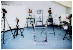 | |
| Fig. 3: | An optoelectronic system |
M1 and M2 are, respectively the mediums of markers (A, B) and (C, D). The ![]() axis is such as:
axis is such as:
We have reference frames built starting from markers fixed on the bones. Calculations of displacements are affected by the errors due to the measurement of the positions of these markers.
The markers being directly related to the osseous structure the theory of finished displacements is well adapted to define the kinematics of the articulation. This method makes it possible to calculate the parameters of an unspecified displacement between two positions. The direction of the axis and the articular amplitude of rotation are then given starting from the operator of finished rotation; for an unspecified movement a succession of axes is then calculated.
Helical axis method: Let us the relative finished displacement of the tibia (index T) compared to the femur (index F) between two positions: A position of reference 1 and one current position i. The co-ordinates of the markers belonging to the solids tibia and femur to each moments expressed in the fixed reference mark (R0) are known. It is possible to define the homogeneous matrices and of rotations ![]() and then deduce the relative matrix of rotation:
and then deduce the relative matrix of rotation:
 |
Where:
| = | Homogeneous matrices. They define the position and the orientation, respectively of reference frames related to the tibia and the femur compared to the reference frames of the laboratory at the moment 1 | |
| = | Matrices of rotation defining the orientation of the reference frames related to the tibia and the femur compared to the reference mark fixes at moment 1 | |
| B, D | = | Origins of the reference frames tibia and femur expressed in the reference mark of the laboratory |
Knowing the position of the two solids at state 1 and state i, we can calculate the parameters of screwing defining finished displacement: ![]() , θ, t. Movement of a solid between two states can be defined by
, θ, t. Movement of a solid between two states can be defined by ![]() , θ, t, These parameters are consisted the direction of the axis of screwing (unit vector
, θ, t, These parameters are consisted the direction of the axis of screwing (unit vector ![]() ), the amplitudes of rotation θ and translation t around and along the axis (Guttierrez and Dimnet, 1994):
), the amplitudes of rotation θ and translation t around and along the axis (Guttierrez and Dimnet, 1994):
 |
With the assumption ![]() representing the immobilization of the reference frame femur for the determination of the relative displacement of the tibia.
representing the immobilization of the reference frame femur for the determination of the relative displacement of the tibia.
The direction of the axis of screwing and the amplitude of relative rotation are expressed using the elements of the matrix ![]() . If rij are the coefficients of this matrix, we have the following relations:
. If rij are the coefficients of this matrix, we have the following relations:
 |
The scalar t which characterizes the translation along of the axis is expressed by the following relation:
Where:
| = | Gives projections of the translation according to three axes of the reference mark tibia |
Position of reference: The technique of screwing defines the angular variations between two positions i and j but the results must correspond to situations known by the clinicians: on the acquisition of the movement can start with a position that is not fully extended or the method of kinematics requires to define the reference position i, the images that it is necessary to identify the position of maximum extension that will be considered as a reference position. In order to know the real inflection of the knee, we were brought to determine it starting from the relative position of 3 markers; the latter are laid out of way such as they remain appreciably in the same plan during the recording. The zero of extension is defined by the alignment of three markers. For the biomecanicians, the parameters of a relative displacement have significance but they are unusable for the clinical applications. For the clinicians angular, displacements of an articulation must be connected to the anatomical axes, this operation of decomposition implies two conditions: The anatomical axes must be known explicitly, the method of analytical decomposition of total rotation must be clearly defined. In this study a protocol was established to describe the anatomical axes from the position of markers on the bones. Moreover, a particular stress was laid on the methods of decomposition which consists of projecting the total rotation obtained by helical axis method on beforehand selected axes to obtain exploitable articular parameters on the clinical level.
Projection: Tibia: The components of the unit vector ![]() are expressed in the reference mark of the tibia in the position of reference. Choose, by convention, the vector
are expressed in the reference mark of the tibia in the position of reference. Choose, by convention, the vector ![]() such as it is directed to the top i.e., K (2)>0. The sign of the angle θ will be given by the sign of (r13-r31). The users are interest by the knowledge of projections of
such as it is directed to the top i.e., K (2)>0. The sign of the angle θ will be given by the sign of (r13-r31). The users are interest by the knowledge of projections of ![]() θ on suitably selected axes. The direction of the vector
θ on suitably selected axes. The direction of the vector ![]() or the amplitude θ does not affect the values of projection.
or the amplitude θ does not affect the values of projection.
Projection: Functional axes: The functional axes materialize the anatomical functions of the articulations. In biomechanics they correspond to the axes of elementary rotations of the human articulations.
For the studies in-vivo, these axes are given thanks to pre-handling. They consist in asking about making pure rotations of each articular group; for each pure rotation a functional axis is given by Guttierrez and Dimnet (1994). In the studies in-vitro, this pre-handling was not possible, the pure movements being difficult to realize, it is necessary to have a motion generating. The functional axes are the directions of what takes place around an elementary rotation of joint groups. For the knee, during walking three rotations co-exist simultaneously, to isolate each rotation of global movement it must first known the functional axes, these axes defined below coincide with assumed anatomical axes defined by clinicians.
For reasons of interpretations private clinic, the vector of relative rotation ![]() θ is not projected on axes related to the same bone (tibia or femur). This vector is projected on a hybrid system of axes utilizing the staff managements (or anatomical) of the two bones:
θ is not projected on axes related to the same bone (tibia or femur). This vector is projected on a hybrid system of axes utilizing the staff managements (or anatomical) of the two bones:
| • | The unit vector of the bending axis |
| • | The unit vector of the clean axis |
The third axis ![]() corresponding to abduction, it is obtained by construction starting from the two first:
corresponding to abduction, it is obtained by construction starting from the two first:
The vector ![]() θ is broken up on these 3 axes according to the relation:
θ is broken up on these 3 axes according to the relation:
where, θf, θr, θa are the amplitudes of inflection, rotation and abduction, respectively.
The articular amplitudes are calculated directly by inversion of the matrix formed starting from the axes of projection. This method is valid for an orthonormal or not. For projection on the functional axes, the system of axes is not perpendicular between-them but the angle formed by the bending axis and the axis of rotation is practically constant. For the clinicians, the bending axis is not related to the tibia but to the femur. This information was used to calculate corresponding projection.
In the hybrid system of axis the anatomical projection axes are independent which are by assumption the functional axes, on the other hand for projection in the reference mark tibia, the axes of projection are orthogonal and selected to represent the anatomical axes as well as possible.
Projection: Axe of abduction floating: This projection is based on the same principle as the preceding one. The vector of total rotation is regarded as a linear combination of elementary rotations around beforehand definite axes. In this type of projection, the axis of abduction is supposed to be unknown and floating. The remainder of the projection of the total amplitude on the rotation and bending axes is regarded as an elementary rotation of amplitude equal to that of abduction and being carried out around the floating axis:
 |
In this case the amplitude of abduction is defined by the standard of the vector ![]() :
:
Expression of the translation: The calculation of the translations by the method of screwing gives unsatisfactory results: The vertical and frontal components did not reproduce the cycle of the movement. No significant difference in the amplitudes of translation in the sagittal plan for a healthy knee and a knee without LCA, this is why we adopted another method concerning calculation of the translations. This one will be presented hereafter. The translation of the knee is obtained by projecting the center of the knee in the reference mark related to the tibia. This point was selected as being that which is the least mobile in the reference mark of the bone for displacements in rotation. That is to say:
![]() is the center of the knee in the reference mark of the laboratory at moment i. This point is supposed in coincidence with the medium of the markers A', B' placed on the femoral condyles. It is projected at every moment (i = 1, N) in the reference mark tibia by the formula:
is the center of the knee in the reference mark of the laboratory at moment i. This point is supposed in coincidence with the medium of the markers A', B' placed on the femoral condyles. It is projected at every moment (i = 1, N) in the reference mark tibia by the formula:
The translation is calculated like the displacement of the center of the knee compared to a position of reference 1:
The vector instantaneous translation ![]() is expressed in the reference mark tibia.
is expressed in the reference mark tibia.
Each component of this vector defines a translation along the axis corresponding of the reference mark tibia.
Sequential method: In mechanics, screwing is useful because it is a synthetic representation of displacement. Its interest is limited with regard to biomechanics. The analysis of the results of screwing in the clinical plan depends on the choice of the axes of projection. The latter determine the values of the components of global rotation. It is interesting to note that the components of the vector ![]() θ of global rotation correspond to simultaneous rotations, contrary with the sequential methods (Euler…) which determine the components of rotation according to the order defined by the sequence.
θ of global rotation correspond to simultaneous rotations, contrary with the sequential methods (Euler…) which determine the components of rotation according to the order defined by the sequence.
We distinguish 2 types of approach: The sequential method with fixed axis (Cardan type RPY: Roll, Pitch, Yaw) and sequential method with mobiles axis (Euler type). The second approach is used in this case. The principle of the method may be thus stated.
The sequence begin with a rotation around one from the fixed axes (that is to say ![]() ), the transform is a reference frame R1 following rotation is carried out around one of the axes of the reference frame R1 which was not in coincidence with an axis of the reference frame fixe R0 the transform is a reference frame R2 finally a rotation around one of the axes of the reference frame R2 which did not remain motionless compared to R1 brings the reference mark in position R3 which, by assumption, is supposed to be identical to the final reference frame RS desired.
), the transform is a reference frame R1 following rotation is carried out around one of the axes of the reference frame R1 which was not in coincidence with an axis of the reference frame fixe R0 the transform is a reference frame R2 finally a rotation around one of the axes of the reference frame R2 which did not remain motionless compared to R1 brings the reference mark in position R3 which, by assumption, is supposed to be identical to the final reference frame RS desired.
Conversely, if two positions of reference mark (R0 and R3) are known, there are always 3 angles which allow the passage of the reference mark R0 to the reference mark R3.
There are several possible sequences of elementary rotations to make pass a reference mark of an initial position R0 to a final position R3, in the sequential methods (of Euler type), the articular amplitudes depend on the order chosen for the axes.
The matrix of relative rotation is defined using the product of the elementary matrices corresponding to 3 successive rotations around independent axes.
The amplitudes of elementary rotations differ if sequence is changed, there are 3! (6) Possible combinations depending on the order chosen to mobilize the plans of orientations. Sequence 132 of axes (![]() ) representing the functional axes of flexion, abduction and rotation own, gives a combination of angles (θf, θa, θr) interpretable in a satisfactory way by the clinicians. It corresponds to a flexion followed by an abduction and finally of a proper rotation:
) representing the functional axes of flexion, abduction and rotation own, gives a combination of angles (θf, θa, θr) interpretable in a satisfactory way by the clinicians. It corresponds to a flexion followed by an abduction and finally of a proper rotation:
  |
The angles (θf, θa, θr) are expressed in radians. rij is components of the matrix ![]() describing the global position of the final reference mark RS compared to the initial reference mark R0 .
describing the global position of the final reference mark RS compared to the initial reference mark R0 .
The Atan 2 function of language FORTRAN takes account of the sign of the numerator and the denominator of the expression of the function arc-tangent in order to obtain an angle defined between -π et π.
RESULTS
On the following figures the values were traced corresponding to the same global movement but by using various techniques of projections (functional axes, axes of the reference frame tibia) with the assumption of simultaneity of projections (helical axis method) and with the assumption of sequential rotations (Sequential method). High repeatability is observed in the shapes of the trajectories: for the same imposed movement, the same angular variations are observed on the curves of bending, own rotation and abduction. Similarly, a coupling is observed between flexion and abduction and flexion and rotation own: when the axial rotation and abduction are minimum position, anatomical specimen is in a position of maximum extension and back positions of maximum axial rotation and abduction corresponds to the maximal flexion.
In the 3 cases of projection and for the method of Euler, the same angular variations (Fig. 4) are observed on the curves of bending and axial rotation (graphs C1, C3). With regard to abduction, we find in each case a different angular variation (graph C2). This can be explained by the orientation of the axis of abduction, whose direction is not identical in the various cases: For the matrix procedure (projection functional axes) the axis of abduction is perpendicular to the plan formed by the axis of axial rotation and the axis of bending. These two axes are not perpendicular to one another. While for projection in the reference mark tibia, the axis of abduction is obtained from two orthogonal axes.
 | |
| Fig. 4: | Different graphs for angular variations |
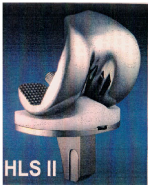 | |
| Fig. 5: | Knee prosthesis |
Projection with the floating axis gives similar results compared to two other projections concerning the angles of inflection and of rotation. For the angle of abduction the results is not considered to be reliable, it is generally non satisfactory. This can be explained by the fact that the axis Za: Axis of abduction calculated with this method can represent an unspecified direction which is far from corresponding to an anatomical axis (graph C4).
Called for proper comparison between different types of knee, the prosthesis stabilised-posterior restore approximately the movement extension-flexion of the safe knee. The regularity of the cycle is more remarkable for the prosthesis knee. The good quality of the design of the prosthesis (Fig. 5) and the conditions of installation may be the cause of this performance. The extension-flexion cycle inversion time is longer in the case of safe knee than in the case of the prosthesis knee. This is due to the fact that the prosthesis has no or a little damping if any: for the safe knee the articulate surfaces and ligaments crossed play a role on the damping of the movement especially on the end of the cycle (graph C5). For knee without LCA, the axial rotation is weaker, it’s about 5° and the cyclic phenomenon is less remarkable (graph C7). The same for the knee without ACL, the cycle of movement is difficult to identify because of the instability of the abduction-adduction movement in dynamic situation (graph C6). It’s important to realise that when the LCA is cut, the amplitude of this rotation is important at rest under static conditions. In movement, the amplitude of this rotation is relatively small, this may be explained by gliding movement of the femur with respect to the tibia and the increase of the pressure efforts is made on the articulation surfaces during the flexion. In my opinion, these 2 factors limit the axial rotation under dynamics condition.
In the case of the tibial translation on the sagital plan, the maximum amplitude is observed for knee without ACL. The observed translations peaks correspond to the instable rapid gliding movement of the femur with respect to the tibia. They are remarkable starting from certain angles of flexion. For the prosthetic knee, the amplitude of translation is nearly null. The fluctuations observed on the graph (C8) are due to the uncertainly of measure system.
CONCLUSION
This article focuses on the kinematics’ study of a knee in three cases: Healthy knee, instrumented prosthesis and without ACL. Work was done on an anatomic specimen (in vitro study) which simulated in vivo conditions: The bending motion is carried continuously and a load of 400 N is applied to the femoral head. The protocol was defined as rigorously as possible so that the experiments can be considered reproducible enough to allow a qualitative comparison. An effort is developed to show the importance of the axes of projection and the method of treatment of joint movement. To be exact, it is necessary to systematically identify the method and the axes of projection when interpreting the results of the kinematics. Two kinematics methods were applied to describe the relative displacement relating the adjacent segments to the knee joint. A particular interest is given to the choice of projection’s axes and the sequence of rotation making it possible to break up the global displacement of the femur compared to the tibia in an exploitable form by clinicians. As far as helical axis method is concerned, projection on functional axes appears most adequate in the decomposition of global rotation. Projection in the tibia mark reference (such as it was defined in the article) gives also good results. For the sequential method with mobile axes, it is essential to specify the order of the sequence. In our application, sequence XZY gives results similar to those obtained by helical axis method with projection on functional axes. This report is undoubtedly an essential complement to this research deals with a first attempt to understand the influence of specific knee pathologies.
REFERENCES
- Argenson, J.N., R.D. Komistek, M. Mahfouz, S.A. Walker, J.M. Aubaniac and D.A. Dennis, 2004. A high flexion total knee arthroplasty design replicates healthy knee motion. Clin. Orthop. Relat. Res., 428: 174-179.
PubMed - Andriacchi, T.P., P.L. Briant, S.L. Bevill and S. Koo, 2006. Rotational changes at the knee after ACL injury cause cartilage thinning. Clin. Orthop. Relat. Res., 442: 39-44.
PubMed - Cheze, L., B.J. Fregly and J. Dimnet, 1995. A solidification procedure to facilitate kinematic analyses based on video system data. J. Biomech., 28: 879-884.
PubMedDirect Link - Duffy, G.P., A.R. Crowder, R.R. Trousdale and D.J. Berry, 2007. Cemented total knee arthroplasty using a modern prosthesis in young patients with osteoarthritis. J. Arthroplasty, 22: 67-70.
PubMed - Frain, P., C. Fontaine and D. D'Hondt, 1984. Constraints of knee ligament trouble meniscofemoral. Study of the internal condylotibial joint. Experimental cinematic method. Rev. Chir. Orthop. Reparatrice Appar. Mot., 70: 361-369.
PubMedDirect Link - Li, G., E. Most, P.G. Sultan, S. Schule, S. Zayontz and S.E. Park, 2004. Knee kinematics with a high flexion posterior stabilized total knee prosthesis: An in vitro robotic experimental investigation. J. Bone Joint Surg., 86-A: 1721-1729.
PubMed - Reuben, J.D., J.S. Rovick, R.J. Schrager, P.S. Walker and A.L. Boland, 1989. Three dimensionnal dynamic motion analysis of the anterior cruciate ligament deficient knee joint. Am. J. Sports Med., 17: 463-471.
CrossRefPubMedDirect Link - Ruby, P. and M.L. Hull, 1993. Response of intersegmental knee loads to foot/pedal platform degrees of freedom in cycling. J. Biomech., 26: 1327-1340.
PubMedDirect Link - Saari, T., J. Uvehammer, L.V. Carlsson, P. Herberts, L. Regrer and J. Karrholm, 2003. Kinematics of three variations of the Freeman-Samuelson total knee prosthesis. Clin. Orthop. Relat. Res., 410: 235-247.
PubMed - Shiavi, R., T. Limbird, M. Frazer, K. Stivers, A. Strauss and J. Abramovitz, 1987. Helical motion analysis of the knee II. Kinematics od ininjured and injured knee during walking and pivoting. J. Biomechanics, 20: 653-665.
PubMed - Stiehl, J.B., D.A. Dennis, R.D. Komistek and P.A. Keblish, 2000. In vivo kinematics comparison of posterior cruciate ligament retention or sacrifice with a mobile bearing total knee arthroplasty. Am. J. Knee Surg., 13: 13-18.
PubMed - Ling, Z.K., H.Q. Guo and S. Boersma, 1997. Analytical study on the kinematic and dynamic behaviors of a knee joint. Med. Eng. Phys., 19: 29-36.
PubMed