
C. Jayakumari
D.G. Vaishnav College, Arumbakkam, Chennai, Tamil Nadu, India
T. Santhanam
D.G. Vaishnav College, Arumbakkam, Chennai, Tamil Nadu, India
Information Technology Journal
Year: 2008 | Volume: 7 | Issue: 2 | Page No.: 386-395


ABSTRACT
A novel technique of intelligent segmentation and classification of exudates for diabetic retinopathy by applying energy minimization method using a recurrent neural network that is an Echo State Neural Network (ESNN) which, yields highly satisfactory results when compared with that of an existing contextual clustering segmentation (CC) is explored in this study. The modular neural network is trained using a set of 30 images consisting of 5 normal images and 25 abnormal images. The trained system has been tested with 5 normal and 20 abnormal images and is found to acquire satisfactory results with 90% (18/20) sensitivity.
PDF Abstract XML References Citation
How to cite this article
C. Jayakumari and T. Santhanam, 2008. An Intelligent Approach to Detect Hard and Soft Exudates Using Echo State Neural Network. Information Technology Journal, 7: 386-395.
DOI: 10.3923/itj.2008.386.395
URL: https://scialert.net/abstract/?doi=itj.2008.386.395
DOI: 10.3923/itj.2008.386.395
URL: https://scialert.net/abstract/?doi=itj.2008.386.395
INTRODUCTION
The human eye is the organ which provides sense of sight. With the help of eyes one can see and interpret the shapes, colors and dimensions of objects in the world by processing the light they reflect or emit. The eye is able to see in the presence of bright or in dim light, but can not see objects in the absence of light. The clarity of one’s vision is characterized as visual acuity which determines how well a person can see. The reduction in its value can lead to several eye disorders. Not all eye problems are minor and some of them even lead to permanent loss of vision like Diabetic retinopathy.
Diabetic retinopathy is a chronic progressive sight-threatening disease of the retinal microvasculature related with the prolonged hyperglycaemia and other conditions linked to diabetes mellitus such as hypertension. Diabetic retinopathy is classified according to the presence or absence of abnormal new vessels as: non-proliferative (background/pre-proliferative) retinopathy, proliferative retinopathy.
Kanski (1994) has explained that the retina is a layer of tissue in the back of the eye that senses light and sends images to the brain. In the center of the nerve tissue is the macula. It provides the sharp, central vision needed for reading, driving and seeing. Retinal disorders affect this vital tissue. They can affect the vision and some can be serious enough to cause blindness and one such disease is known as Diabetic Retinopathy.
Lot of research work has been done focusing on automatic segmentation and classification of the affected eye based on the type of exudates. Nguyenl et al. (1996) have presented a robust system for grading diabetic retinopathy using a complex neural network structure which would take into account multiple windows and shows lesions in multiple photographic fields with noisy images. The results are compared with various retinopathy severity scales to classify the diseases. Hsu et al. (2006) exercised the role of domain knowledge to mine the retinal hard exudates. The normalization is accomplished by median filtering procedure. The dynamic clustering technique has been used to perceive the lesion and then domain knowledge to recognize the true hard exudates. Osareh et al. (2002) has used histogram equalization, contrast enhancement technique for normalization and fuzzy c-means for segmentation. The classifications of lesions are performed using various neural network classifiers like Linear Delta Rule (LDR), K-Nearest Neighbours (KNN). Walter et al. (2002) extracted the exudates using their high grey level variation and their contours are determined by means of morphological reconstruction techniques. The detection of the optic disc has been achieved by means of morphological filtering techniques and the watershed transformation. After normalizing and performing contrast enhancement, a coarse and fine segmentation using fuzzy c-means technique have been employed followed by three layer perceptron neural network for classification by Osareh et al. (2003), they also have experimented with a number of color spaces. Exudates are extracted by the combined region growing and edge detection, disk boundary detection and fovea localization, respectively. Chutatape and Li (2003) has attempted two step improved fuzzy c-means in Luv color space to segment candidate bright lesion area after the preprocessing stage. A hierarchical support vector machine classification structure is applied to classify bright non-lesion areas by Zhang (2005). Carnimeo and Giaquinto (2006) have investigated with a neurofuzzy technique for contrast enhancement. The fuzzy rules are implemented using a sparsely-connected (4x4) cell Hopfield-type neural network. Enhanced contrast images properly segmented to isolate suspected areas in binary by making use of thresholding technique and neural network. Kahai et al. (2006) has done the classification based on Bayesian framework, namely, the likelihood ratio test, maximum a posteriori detector and Bayes detector. A machine learning program that can differentiate between drusen and soft exudates were developed by Niemeijer et al. (2007). Walter et al. (2002) has used grey level variation to detect exudates. Akara et al. (2007) has initially segmented the image using fuzzy c-means and later using morphological reconstruction by considering four features, namely intensity, standard deviation on intensity, hue and adapted edge. Xiaohui and Chutatape (2004) has employed local contrast enhancement, two-step improved fuzzy C-means in Luv color space to segment candidate bright-lesion areas and finally, a hierarchical Support Vector Machine (SVM) has been used to classify bright non-lesion areas, exudates and cotton wool spots.
Problem definition: The main objective of this research is to segment different types of exudates and classify them for suitable diagnosis, using an echo state neural network (ESNN). The segmentation of exudates by ESNN is compared with the segmentation performance of conventional contextual clustering. Representative features of the image are collected using contextual clustering. The proposed ESNN method learns the features of 35 representative images to produce a set of final weights. Theses final weights are used to segment a test image and classify the exudates using ESNN.
Schematic flow diagram: The sequence of steps required for the paramount segmentation and classification of hard and soft exudates by implementing an ESNN has been given in Fig. 1. The histogram distribution of the fundus images has to be uniform for the achievement of attractive segmentation process. Hence an image is taken as reference image and the intensity histogram of other images is made more or less equal to the reference image by finding the minimum and maximum intensity values.
Image contrasting is done for all the images to enhance the image. Features of the images are then obtained from the moving window and used as an input for the ESNN along with initial random weights and labeled as target values.
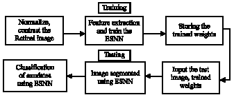 | |
| Fig. 1: | Schematic diagram of the intelligent segmentation |
After training the ESNN, a set of final weights are obtained and stored in a file. During the process of testing, a test image is normalized to the reference image which is followed by histogram equalization and contrast enhancement. ESNN performs segmentation by using the final weight values arrived during training phase and finally classification of exudates is performed.
IMAGE SEGMENTATION
Image segmentation is a subjective and context-dependent cognitive process. It implicitly includes not only the detection and localization but also the delineation of the activated region. In medical imaging field, the precise and computerized delineation of anatomic structures from image data sequences is still an open problem. Countless methods have been developed, but as a rule, user interaction cannot be negated or the method is said to be robust only for unique kinds of images.
Contextual Clustering (CC): Contextual Clustering is a technique to perform segmentation into two classes, a background class ω0 and an alternative class ω1 by hypothesis testing simultaneously utilizing neighborhood information. The true distribution of the class ω0 is known to be the standard normal N(0,1). The distribution of class ω1 values is unknown. The classification can be one-sided hypothesis test, accepting null hypothesis that the pixel belongs to ω0 whenever the pixel intensity zi is smaller than a predefined threshold Tcc and otherwise rejecting the null hypothesis and thus classifying pixel to class ω1. In order to utilize neighbourhood information, an artificial distribution for class ω1 is introduced. The steps involved in contextual clustering are given as follows (Salli et al., 2001).
Step 1: Define a decision parameter Tcc(positive) and the weight of neighbourhood information β (positive). Let Nn to be the total number of pixels in the neighbourhood. Let zi be the intensity value of pixel i.
Step 2: Classify pixels with zi > Tcc to ω1 and other pixels to ω0. Store the classification to variables Co and C1.
Step 3: For each pixel i, count the number of pixels, ui, belonging to class ω1 in the neighborhood of pixel i. Assume that the pixels outside the image belong to ω0.
Step 4: Classify pixels with
to ω1 and other pixels to ω0. Store classification variable to C2.
Step 5: If C2 = C1 and C2 = C0 stop else store C1 in C0 and C2 in C1 and go to step 3.
Echo State Neural Network (ESNN): An Artificial Neural Network (ANN) is an abstract simulation of a real nervous system that contains a collection of neuron units, communicating with each other via axon connections. Such a model bears a strong resemblance to axons and dendrites in a nervous system. Due to this self-organizing and adaptive nature, the model offers potentially a new parallel processing paradigm. This model could be more robust and user-friendly than the traditional approaches. ANN can be viewed as computing elements, simulating the structure and function of the biological neural network. These networks are expected to solve the problems, in a manner which is different from conventional mapping. Neural networks are used to mimic the operational details of the human brain in a computer. Neural networks are made of artificial ‘neurons’, which are actually simplified versions of the natural neurons that occur in the human brain. A neural architecture comprises massively parallel adaptive elements with interconnection networks, which are structured hierarchically.
Artificial neural networks are computing elements which are based on the structure and function of the biological neurons (Lippmann, 1987). These networks have nodes or neurons which are described by difference or differential equations. The nodes are interconnected layer-wise or intra-connected among themselves. Each node in the successive layer receives the inner product of synaptic weights with the outputs of the nodes in the previous layer (Rumelhart et al., 1986). The inner product is called the activation value.
Dynamic computational models require the ability to store and access the time history of their inputs and outputs. The most common dynamic neural architecture is the time-delay neural network that couples delay lines with a nonlinear static architecture where all the parameters (weights) are adapted with the backpropagation algorithm.
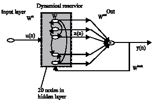 | |
| Fig. 2: | An echo state neural network (ESNN) |
Recurrent Neural Networks (RNNs) implement a different type of embedding that is largely unexplored. One of the main practical problems with RNNs is the difficulty to adapt the system weights. Backpropagation through time and real-time recurrent learning, have been proposed to train RNNs. These algorithms suffer from computational complexity, resulting in slow training, complex performance surfaces, the possibility of instability and the decay of gradients through the topology and time. The problem of decaying gradients has been addressed with special processing elements (PEs).
ESNNs (Jaeger, 2001) possesses a highly interconnected and recurrent topology of nonlinear PEs that constitutes a reservoir of rich dynamics and contains information about the history of input and output patterns. The topology of the network is shown in Fig. 2. The outputs of this internal PEs (echo states) are fed to a memory less but adaptive readout network (generally linear) that produces the network output. The interesting property of ESNN is that only the memory less readout is trained, whereas the recurrent topology has fixed connection weights. This reduces the complexity of RNN training to simple linear regression while preserving a recurrent topology, but obviously places important constraints in the overall architecture that have not yet been fully studied.
The echo state condition is defined in terms of the spectral radius (the largest among the absolute values of the eigenvalues of a matrix, denoted by (|| ||) of the reservoir’s weight matrix (|| W || < 1). This condition states that the dynamics of the ESNN is uniquely controlled by the input and the effect of the initial states vanishes. The current design of ESNN parameters relies on the selection of spectral radius. There are many possible weight matrices with the same spectral radius.
ESNN is composed of two parts (Jaeger, 2002a): a fixed weight (|| W || < 1) recurrent network and a linear readout. The recurrent network is a reservoir of highly interconnected dynamical components, states of which are called echo states. The memory less linear readout is trained to produce the output (Jaeger, 2002b). The recurrent discrete-time neural network is given in with M input units, N internal PEs and L output units.
The value of the input unit at time n is:
u(n) = [u1(n), u2(n),..., uM(n)]T, | (1) |
The internal units are
x(n) = [x1(n), x2(n),..., xN(n)]T and | (2) |
Output units are
y(n) = [y1(n), y2(n),..., yL (n)]T. | (3) |
The connection weights are given
| • | In an NxM weight matrix |
| • | In an NxN matrix |
| • | In an LxN matrix |
| • | In an NxL matrix |
Where:
M=No. of neurons in the input layer
N=No. of neurons in the hidden layer
L =No. of neurons in the output layer
The activation of the internal PEs (echo state) is updated by using the relation
x(n + 1) = f(Win u(n + 1) + Wx(n) +Wbacky(n)), | (4) |
Where:
f=(f1, f2,..., fN) are the internal PEs’ activation functions.
All fi’s are hyperbolic tangent functions
The output from the readout network is computed as follows:
y(n + 1) = fout(Woutx(n + 1)), | (5) |
Where:
fout=(f1out, f2out,...., fLout) are the output unit’s of nonlinear functions.
The ESNN topology specified in this study is {2xNo. of reservoirs x1}, where two nodes are in the input layer, one in the output layer and any number of reservoirs in the hidden layer. The connections between input-hidden layers, hidden-output layer are initialized with random numbers. The training of the ESNN is done with choosing initial random weights in a range of 0.25 to 0.55. The random weights are chosen within a small range for easier quicker settlement of final weights and also to prevent the network from further oscillation.
Implementation of segmentation using ESNN: To obtain the trained weights by training the ESNN
Step 1: Find the statistical features of the image (i.e.,) the features are properties of moving window.
Step 2: Fix the target values.
Step 3: Set the No. of inputs, No. of reservoirs, and No. of outputs.
Step 4: Initialize connection matrices-using random weights for
| No. of reservoirs versus No. of inputs, No. of outputs versus No. of reservoirs, No. of reservoirs versus No. of reservoirs. |
Step 5: Determine values of matrices less than a threshold for updating the weights.
Step 6: Normalize the reservoir matrix by finding its eigen value.
Step 7: The initial state matrix is updated with tanh() function. The inputs for the tanh() function are:
{input pattern X weights between input and hidden layer +desired output X weights between output and hidden layer +normalized reservoir matrix}
Step 8: Store the weight matrices.
Implementation of ESNN for segmentation of retinopathy image using the trained weights of ESNN
Step 1: The trained weights are given as inputs.
Step 2: Apply the statistical features of retinopathy image obtained from the moving window.
Step 3: Process the inputs with the trained weights.
Step 4: Employ transfer function to get the output of the ESNN.
Step 5: Set threshold and segment the image.
Over all algorithms for training and testing:
| • | Obtain the statistical feature of the image from the moving window. |
| • | Train the ESNN with the inputs and target outputs. Trained weights are obtained once all the patterns are presented to the ESNN |
| • | Test the ESNN with a new image and segment the image. |
| • | Remove the Optic disc from the segmented image. |
| • | Classify the exudates with ESNN. The input features obtained using the softwre matlab. |
EXPERIMENTAL RESULTS
The automated exudate identification system has been developed using color retinal images obtained from one of the popular eye clinics in Chennai (India).
According to the National Screening Committee standards, all the images are obtained using a Canon CR6-45 Non-Mydriatic (CR6-45NM) retinal camera. A modified digital back unit (Sony PowerHAD 3CCD color video camera and Canon CR-TA) is connected to the fundus camera to convert the fundus image into a digital image. The digital images are processed with an image grabber and saved on the hard drive of a Windows 2000 based Pentium -IV.
The sample images of normal and abnormal type are shown in Fig. 3.
Representative exudates are isolated from the original retinopathy images to create exudates templates which are shown in Fig. 4 and 5. It can be noted that there is a variation in image content between hard and soft exudates with respect to segmentation process.
Statistical features for the hard and soft templates and their values have been determined using Matlab are given below.
Convex area: The number of pixels in 'ConvexImage'. This property is supported only for 2-D input label matrices.
Solidity: The proportion of the pixels in the convex hull that are also in the region. Computed as Area/ConvexArea. This property is supported only for 2-D input label matrices.
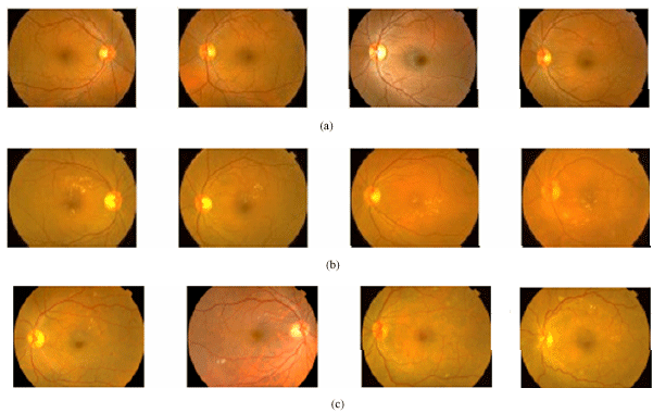 | |
| Fig. 3: | Sample images considered for implementing ESNN. (a) Normal images, (b) Images with hard exudates and (c) Images with soft exudates |
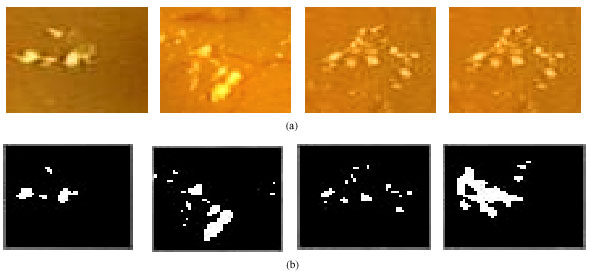 | |
| Fig. 4: | Segmented pictures of hard exudates. (a) Sample hard exudates and (b) Segmentes hard exudates by ESNN |
 | |
| Fig. 5: | Segmented pictures of soft exudates. (a) Sample soft exudates and (b) Segmentes soft exudates by ESNN |
Orientation: The angle (in degrees) between the x-axis and the major axis of the ellipse that has the same second-moments as the region. This property is supported only for 2-D input label matrices.
Filled area: The number of on pixels in FilledImage.
Segmentation outputs of hard and soft outputs for hard and soft exudates
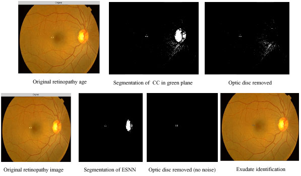
Hard exudate intermediate outputs using contextual clustering and ESNN: In Fig. 6 different stages of outputs of CC and ESNN are given. The entire image processing included here involves normalizing, histogram equalization, segmentation.
Figure 6 shows sequence of outputs for the image with hard exudates. The hard exudates are found in the centre of the retinopathy image. The first row indicates the outputs of CC and the second row shows the outputs of ESNN. In column 1, the original image is shown. Column 2 shows the segmented image. During training of ESNN, 30 reservoirs for hard exudates and 10 reservoirs for soft exudates have been used. The segmented image of CC shows more noise. The optic disc from the image is removed by using a circular mask. Since the noise is present in CC segmented image, it is not carried out further (column 4). In the case of ESNN, further processing is done by searching the exudates available using moving window (column 4).
 | |
| Fig. 6: | Comparison of segmentation outputs of CC and ESNN for hard exudate |
The imfeatures such as ConvexArea, Solidity, Orientation, FilledArea are calculated for the moving window during the classification process and are given as into to the ESNN which classifies it as exudate or not.
In Table 1, set of sample features obtained during the movement of window are given. During this process, intensity values in the moving window are added and given in the first column. This gives the weight of moving window. The values are normalized by 1000. One can choose mean or total intensity or Minimum and Maximum value of the window. However the mean will not show the range of values inside the window. The contextual values calculated using step 4 of section 5 is given in second column of Table 1. The third column contains a target value of 0.1 if the contextual value is less than the specified threshold (Hard = 165 and Soft = 120) and 0.9 if the contextual value is greater than the threshold given. These features will be further used to train ESNN to obtain set of trained weights as given in Table 2.
The ESNN is trained with 2x30x1 topology. The network is initialized with random weights. During the process of training, the weights are updated using the pseudo inverse of different states. The network is stopped once all the patterns are presented for training (column 1 and column 3 of each row from Table 1). Based on the size of moving window (bs) for a given size of R X C images, the no of patterns generated will be total number of overlapping square window:
[R-(bs-1)]+[C-(bs-1)] | (6) |
| Table 1: | Sample set of features |
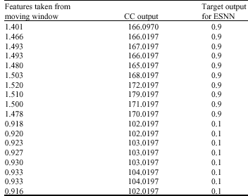 | |
Where:
| bs | = | Size of square window |
| R | = | No. of rows in an image |
| C | = | No. of columns in the image |
As the neural network is used to learn the pattern, only representative patterns are chosen using the Eq. 7. Selection of patterns for training the neural network is important as they should be representative of all the patterns collected. Statistical techniques have been used to select the patterns out of given number of patterns collected during the experiment. Patterns are selected with maximum variance VEi2 selected. The maximum VEi2 of a pattern is found from the equation:
 | |
| Fig. 7: | Outputs of soft exudates using CC and ESNN |
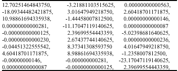
| Table 2: | Trained weights obtained from training ESNN for 30 nodes in the hidden layer |
 | |
 | (7) |
Where:
| x | = | The feature value |
| p | = | The pattern |
| nf | = | No. of features and |
| LL | = | No. of patterns and pi is the pattern number |
One hundred patterns are presented similar to values shown in Table 1 for training ESNN. A set of trained weights are given in Table 2 for hard exudates.
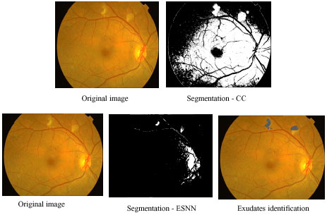
Soft exudate intermediate outputs using contextual clustering and ESNN: Figure 7 demonstrate the series of outputs for the image with soft exudates. The first row indicates the outputs of CC and the second row shows the outputs of ESNN. The first column shows the original image, second column depicts the outputs of segmented image. The segmented image of CC shows more noise. Disc from the image is removed by using a circular mask. Since the noise is present in CC, segmented image it is not carried out further for exudates classification.
 | |
| Fig. 8: | Threshold setting for hard exudate |
In the case of ESNN, further processing is done by searching the exudates available using moving window. The imfeatures are calculated for the moving window and these are given as inputs for the trained ESNN which classifies segmented objects as exudates or not.
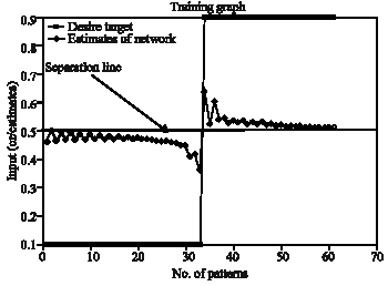
Figure 8 gives the performance of ESNN training. The desired target and the estimated target values are given. In practice the estimated should follow the profile of desired target. However the separation line indicates the threshold to be set during segmentation of the image. The performance of the graph is based on the number of reservoirs. The horizontal separation line indicates the approximate threshold (0.49) used for segmenting the image. If the output of ESNN is less than 0.49, a vale of 0 is put in the image matrix otherwise 255. This appears to be a segmented image.
 | |
| Fig. 9: | Threshold setting for soft exudate |
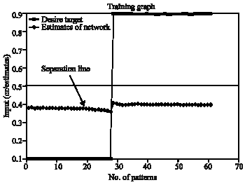
The Fig. 9 shows the performance of ESNN training and threshold setting . The approximate threshold value chosen for segmentation is 0.38. The desired target and the estimated values are given. There is a clear demarcation between two classes. The performance of the graph is based on the number of reservoirs and 10 reservoirs are used in this study for soft exudates segmentation.
CONCLUSION
The main focus of this study is on segmenting the diabetic retinopathy image to extract and classify hard and soft exudates using echo state neural network. The performance classification of exudates has been carried out with template matching and CC is not up to the satisfactory level only in the case of very poor images. The proposed ESNN segmentation segments and classifies the exudates even better in adverse image conditions. The ESNN segments much better than the CC and hence spurious noise is automatically removed to the maximum extent. Classifications of the exudates have been done by ESNN algorithm.
REFERENCES
- Akara, S., B. Uyyanonvara and Sirindhorn, 2007. Automatic exudates detection from diabetic retinopathy retinal image using fuzzy c-means and morphological methods. Proceedings of the 3rd Lasted International Conference Advances in Computer Science and Technology, April 2-4, 2007, Thailand, pp: 559-640.
- Chutatape, O. and L. Huiqi, 2003. A model-based approach for automated feature extraction in fundus images. Proceedings of the 9th International Conference on Computer Vision, October 13-16, 2003, Nice, France, pp: 394-399.
CrossRefDirect Link - Jaeger, H., 2002. Tutorial on training recurrent neural networks, covering BPPT, RTRL, EKF and the "echo state network" approach. GMD Report 159, German National Research Center for Information Technology, pp: 48. http://minds.jacobs-university.de/sites/default/files/uploads/papers/ESNTutorialRev.pdf.
- Kahai, P., K.R. Namuduri and H. Thompson, 2006. A decision support framework for automated screening of diabetic retinopathy. Int. J. Biomed. Imaging., 2006: 1-8.
CrossRefDirect Link - Lippmann, R., 1987. An introduction to computing with neural nets. IEEE ASSP Mag., 4: 4-22.
CrossRefDirect Link - Nguyenl, H.T., M. Butler, A. Roychoudhryl, A.G. Shannonl, J. Flack and P. Mitchell, 1996. Classification of diabetic retinopathy using neural networks. Proceedings of the 18th Annual International Conference of the IEEE Engineering in Medicine and Biology Society, October 31-November 3, 1996, Amsterdam, pp: 1548-1549.
CrossRefDirect Link - Niemeijer, M., B. van Ginneken, R.S. Russell, S.A. Maria, S. Schulten and D. Michael, 2007. Automated detection and differentiation of drusen, exudates and cotton-wool spots in digital color fundus photographs for diabetic retinopathy diagnosis. Invest. Ophthalmol. Visual Sci., 48: 2260-2267.
CrossRefPubMedDirect Link - Osareh, A., M. Mirmehdi, B. Thomas and R. Markham, 2002. Classification and localisation of diabetic-related eye disease. Lecture Notes Comput. Sci., 2353: 502-516.
Direct Link - Osareh, A., M. Mirmehdi, B. Thomas and R. Markham, 2003. Automated identification of diabetic retinal exudates in digital colour images. Br. J. Ophthalmol., 87: 1220-1223.
PubMedDirect Link - Salli, E., J.H. Aronen, S. Savolainen, A. Korvenoja and A. Visa, 2001. Contextual clustering for analysis of functional MRI data. IEEE Trans. Med. Imag., 20: 403-414.
CrossRefDirect Link - Walter, J., C. Klein, P. Massin and A. Erginay, 2002. A contribution of image processing to the diagnosis of diabetic retinopathy-detection of exudates in color fundus images of the human retina. IEEE Trans. Med. Imaging., 21: 1236-1243.
CrossRefPubMedDirect Link - Xiaohui, Z. and A. Chutatape, 2004. Detection and classification of bright lesions in color fundus images. Proceedings of the International Conference Image Processing, October 24-27, 2004, Singapore, pp: 139-142.
CrossRefDirect Link - Zhang, X., 2005. Top-down and bottom-up strategies in lesion detection of background diabetic retinopathy. Proceedings of the Computer Society Conference on Computer Vision and Pattern Recognition, June 20-25, 2005, OPAS Chutatape School of Electrical and Electronic Engineering Nanyang Technological University, Singapore, pp: 422-428.
CrossRefDirect Link