
Bingqun Ren
School of Economics and Finance, Xi`an Jiaotong University, China
Weizhou Zhong
School of Economics and Finance, Xi`an Jiaotong University, China
Information Technology Journal
Year: 2011 | Volume: 10 | Issue: 10 | Page No.: 1908-1916


ABSTRACT
As a novel optimization method, chaos has gained lots of attentions and applications in the past few years. Chaos movement can go through all states unrepeated according to the rule of itself in some area. It was introduced into the optimization strategy to accelerate the optimum seeking operation in this study. A chaos based particle swarm optimization strategy was developed to solve multi-objective optimization problems. The proposed approach is validated using several benchmark test functions and metrics on evolutionary multi-objective optimization. Results demonstrate the effectiveness and efficiency of the proposed strategy and that can be considered a viable alternative to solve multi-objective optimization problems.
PDF Abstract XML References Citation
Received: March 13, 2011;
Accepted: July 24, 2011;
Published: September 19, 2011
How to cite this article
Bingqun Ren and Weizhou Zhong, 2011. Multi-objective Optimization using Chaos Based PSO. Information Technology Journal, 10: 1908-1916.
DOI: 10.3923/itj.2011.1908.1916
URL: https://scialert.net/abstract/?doi=itj.2011.1908.1916
DOI: 10.3923/itj.2011.1908.1916
URL: https://scialert.net/abstract/?doi=itj.2011.1908.1916
INTRODUCTION
Multi-objective Optimization Problems (MOPs) are very common in the real world, especially in engineering applications, like production scheduling, design of complex software system and potential function parameter optimization (Coello et al., 2004; Parsopoulos and Vrahatis, 2002; Ahmed and Zamli, 2011; Hernane et al., 2010). These problems involve optimizing multiple competing and incommensurable criteria that reflect various design specifications and constraints. The use of evolutionary algorithms for multi-objective optimization has significantly grown in recent years (Coello et al., 2004; Zitzler et al., 2003; Chen, 2011). The most common used population-based evolutionary computation techniques are inspired by the evolution of nature.
Particle Swarm Optimization (PSO) is a relatively recent heuristic technique motivated from the simulation of social behavior (Lu and Chen, 2011). PSO has been shown to offer higher convergence speed for multi-objective optimization problems as compared to canonical evolutionary algorithms. The ability to handle complex problems, involving features such as discontinuities, multimodality, disjoint feasible spaces and noisy function evaluations, reinforces the potential effectiveness of PSO in MOPs (Fonseca and Fleming, 1995; Kennedy and Eberhart, 1995). Many PSO based optimizations for MOPs have been developed (Coello et al., 2004; Liu et al., 2007; Zitzler et al., 2002; Deb et al., 2002; Deb, 1999; Cui et al., 2006) but the experimental effect depends on the initial population distribution greatly. It cannot get acceptable results when the distribution doesn’t reflect the population well.
Chaos is one of the most popular phenomenon that exist in nonlinear system, whose action is complex and similar to that of randomness. Chaotic variables can go through all states in certain ranges according to their own regularity without repetition. Due to the ergodic and dynamic properties of chaos variables, chaos search is more capable of hill-climbing and escaping from local optima than random search and thus has been applied to the optimization (Zuo and Fan, 2006). It is now widely recognized that chaos is a fundamental mode of motion underlying almost natural phenomena. Given an energy or cost function, a chaotic dynamic system may eventually reach the global optimum or its best approximation with high probability. Chaos was introduced into the optimization strategy to accelerate the optimum seeking operation. In this study, a chaos based PSO strategy MCPSO was developed to solve MOPs.
Multi-objective optimization: The MOP methodology is to finding optimal solutions to multivariate problems with multiple but often conflicting, objectives (Fonseca and Fleming, 1995; Yang et al., 2009). In most cases, it’s impossible to find the global optimal at the same time for all objectives. The family of solutions is composed of all those potential solutions such that the components of the corresponding objective vectors cannot be all simultaneously improved. The goal of MOP is to provide a set of Pareto optimal solutions to the mentioned problem (Fang et al., 2011).
General MOPs can be defined as following. Let X be an n-dimensional search space and fi (x), i = 1,…, m be m objective functions defined over X. Supposing:
| (1) |
be p inequality constraints, the MOP can be described as finding a vector:
| (2) |
that satisfies the constraints and optimizes the vector function:
| (3) |
Let p = (p1,…, pm) and q = (q1,…, qm) be two vectors. It means that p dominates q if and only if pi≤qi, i = 1,…, m and pi<qi for at least one member. It’s defined as Pareto dominance. A solution ![]() is said to be Pareto optimal if for every
is said to be Pareto optimal if for every ![]() , either:
, either:
| (4) |
or, there is at least one i = 1,…, m such that:
| (5) |
That is to say,![]() is Pareto optimal if there exists o feasible vector
is Pareto optimal if there exists o feasible vector ![]() which would decrease some criterion without causing a simultaneous increase in at least one other criterion. There is not a solution y such that f (y) dominates f (x) (Parsopoulos and Vrahatis, 2002).
which would decrease some criterion without causing a simultaneous increase in at least one other criterion. There is not a solution y such that f (y) dominates f (x) (Parsopoulos and Vrahatis, 2002).
The set of all Pareto optimal solutions of an MOP is called Pareto optimal set and it can be presented by P*. The Pareto front is defined as follow:
| (6) |
A Pareto front is called convex if and only if:
| (7) |
And it is called concave if and only if:
| (8) |
In the general case, it is impossible to find an analytical expression of the line or surface that contains these points. The aim of an Evolutionary Multi-objective Optimization (EMO) is to find a set of Pareto-optimal solutions approximating the true Pareto-optimal front.
Chaos based PSO: PSO is a population based search strategy where individuals, considered as particles, are grouped into a swarm. Each particle represents a potential solution to the optimization problem and each particle has its own fitness value and velocity. These particles fly through the n-dimensional problem space by adjusting their positions and velocities in search space according to their own historical experiences and that of neighboring particles.
In order to handle multi-objective optimization problems, the standard PSO must be modified before being used on MOPs. There have been developed several methods that applied PSO on MOP (Coello et al., 2004; Liu et al., 2007; Parsopoulos and Vrahatis, 2002). The most well known is that Coello developed a grid-based nBest selection process (Coello et al., 2004). In this study, a different chaos optimization strategy was used to handle multiple objectives. The population was disarranged using chaos when it stuck in the local optimum. After several rounds of running, multiple optimums were founded.
Chaos optimization strategy: Chaos has three important dynamic properties: the sensitive dependence on initial conditions, the intrinsic stochastic property and ergodicity. Chaos is in essence deeply related with evolution. In chaos theory, biologic evolution is regarded as feedback randomness, while this randomness is not caused by outside disturbance but intrinsic element (Tong et al., 1999). The chaos based PSO strategy is proposed by integrating chaos optimization algorithm and PSO algorithm. First, the solution space of the optimization problem is mapped to the ergodic space of chaotic variables and thus optimization variables are represented by chaotic variables which are coded into a particle. Then, taking full advantages of the ergodic and stochastic properties of chaotic variables, a chaos search is performed in the neighborhoods of particles to exploit the local solution space and the motion of chaotic variables in their ergodic space is used to explore the whole solution space. Detailed operations of the MCPSO are developed as follows.
Step 1: Initialization: The chaotic variables are generated using classic Logistic mapping equation defined by:
| (9) |
where, L is a control parameter which is between 0 and 4.0 (Moon, 1992). If L ε(3.56, 4.0), then the above system enters into a chaos state and the chaotic variable x is produced. Given arbitrary initial value that is in (0, 1) but not equal with 0.25, 0.5 and 0.75, chaos trajectory will search non-repeatedly any point in the neighborhoods of particles by iteration. Utilizing the chaos characteristic, it can get n chaos variables of different orbits by setting n different initial values to xk in Eq. 9.
Step 2: Solution space transformation: Each chaotic variable corresponds to an optimization particle variable. The range of chaotic variables is (0, 1) and maybe different from that of optimization variables. It can be solved by mapping the ergodic space of the chaos system to the solution space of the optimization problem by Eq. 10:
| (10) |
where, ![]() is the ith optimization variable of the problem and xi is the ith chaotic variable. The continuous function of the optimization problem is treated as the objective function and the particles can be calculated.
is the ith optimization variable of the problem and xi is the ith chaotic variable. The continuous function of the optimization problem is treated as the objective function and the particles can be calculated.
Step 3: Chaotic search in particle neighborhoods: Each particle i has a position defined by Xi = (xi1, xi2,…, xin) and a velocity defined by Vi = (vi1, vi2,…, vin) in the variable space. Each particle has its own best position Pid, corresponding to the personal best objective value obtained so far. The global best particle is denoted by Pgd which represents the best particle found so far. The velocity and position of each particle i is updated as below:
| (11) |
where,
is a chaotic vector and ![]() is the value of the jth chaotic variable at the kth iteration. G1 and G2 are constants called acceleration coefficients, ω is the inertia weight of the particle, r1 and r2 are random numbers uniformly distributed in the range of (0,1). λ is a constriction factor which controls and constricts the chaotic range.
is the value of the jth chaotic variable at the kth iteration. G1 and G2 are constants called acceleration coefficients, ω is the inertia weight of the particle, r1 and r2 are random numbers uniformly distributed in the range of (0,1). λ is a constriction factor which controls and constricts the chaotic range. ![]() is a chaotic vector whose ergodic space is a m-dimensional hypercube. When the chaotic vector xk+1 updates in its ergodic space through chaotic iteration,
is a chaotic vector whose ergodic space is a m-dimensional hypercube. When the chaotic vector xk+1 updates in its ergodic space through chaotic iteration,![]() updates in the neighborhood of xid to perform chaotic search.
updates in the neighborhood of xid to perform chaotic search.
Convergence analysis: Let x3 = agr min f (x) be the logistic mapping used in the optimization search. ![]() is the solution list produced by MCPSO,
is the solution list produced by MCPSO, ![]() is the solution list produced by chaos. For I≤j, it can get
is the solution list produced by chaos. For I≤j, it can get ![]() is a convergence list and
is a convergence list and ![]() is also a convergence list according to converging and approximating theorem (Yadong and Shaoyuan, 2002).
is also a convergence list according to converging and approximating theorem (Yadong and Shaoyuan, 2002).
Metrics of performance: In the case of multi-objective optimization problem, comparing different optimization techniques involves the notion of performance metrics. Zitzler et al. (2003) suggested an infinite number of performance metrics to compare two or more solutions. In this study, the coverage of two sets, the convergence metric and spacing metric were taken into consideration in order to provide a quantitative assessment (Deb et al., 2002; Heng et al., 2006).
Let A, B be two approximate Pareto-optimal sets. The coverage of two sets gives how many decision vectors in B are dominated by A. The function Ic maps the ordered pair (A, B) to the interval (0,1):
| (12) |
where, ≥ means weakly dominate. The value Ic (A, B) means no decision vector in B is weakly dominated by A.
The convergence metric represents the gap between the set of approximate Pareto-optimal solutions (Pfapp, ai εPfapp) and the true Pareto-optimal fronts (Pftrue, ai εPftrue). For each point ai in PFapp, the smallest normalized euclidean distance to PFtrue is given by:
| (13) |
where, ![]() and
and ![]() are the maximum and minimum values of the m-th objective in PFtrue, respectively and k is the number of objective functions. The convergence metric is the average value of the normalized distance for all points in Pfapp:
are the maximum and minimum values of the m-th objective in PFtrue, respectively and k is the number of objective functions. The convergence metric is the average value of the normalized distance for all points in Pfapp:
| (14) |
The metric of spacing desires to measure the spread distribution of vectors throughout the non-dominated vectors found so far. It gives an indication of how evenly the solutions are distributed in objective space. This metric is defined as:
| (15) |
where, ![]() is the average value of all dI.
is the average value of all dI.
Benchmark problems and experimental results: For multi-objective optimization problems, the benchmark problems should possess several features such as multimodality, convexity, discontinuity and non-uniformity which may challenge the algorithms’ capability to converge or to preserve good population diversity (Deb et al., 2002). In this study, CMOPSO (Coello et al., 2004), SPEA2 (Zitzler et al., 2002) and NSGA-II (Deb et al., 2002) were compared with MCPSO in solving six well-known multi-objective optimization benchmark problems. These problems include three low-dimensional problems (DEB, FON and KUR) and three ZDT problems (ZDT1, ZDT2 and ZDT3) (Deb et al., 2002). These problems pose sufficient difficulty to impede the ability in searching for the Pareto optimal solutions and have been applied by many researchers to examine their proposed algorithms (Liu et al., 2007; Parsopoulos and Vrahatis, 2002). The definitions of these six problems are summarized in Table 1.
The group of ZDT benchmark problems defined below is structured in the same manner and consists of three functions fi, g and h.
| (16) |
where, ![]() . The function f1 is a function of the first decision variable only, g is function of the remaining n-1 variables and the parameters of h are the function values of f1 and g.
. The function f1 is a function of the first decision variable only, g is function of the remaining n-1 variables and the parameters of h are the function values of f1 and g.
The first three low-dimensional benchmark functions (DEB, FON and KUR) are simple in scale. They do not have mathematical defined Pareto-optimal fronts. However, their approximate Pareto-optimal fronts have been illustrated in some literature (Deb, 1999). The other three ZDT problems have 30 decision variables. Their Pareto-optimal fronts illustrated by a set of 200 uniform points are shown in Fig. 1. The Pareto-optimal fronts of the three ZDT problems have been mathematically defined by Zitzler et al. (2003).
A population of size 100 and archive size 100 are used in four algorithms, 15 bits for each variable in SPEA2 and NSGA-II, real number representation in CMOPSO and MCPSO. The crossover method is uniform crossover and the crossover rate is 0.85 in SPEA2 and NSGA-II. The number of evaluations is 20,000 for all algorithms. The other parameters are selected according to the proposed literature (Coello et al., 2004; Liu et al., 2007; Zitzler et al., 2002; Deb et al., 2002). Twenty independent simulation runs were performed for each algorithm on each test problem in order to study the statistical performance. Each test problem was initialized with a random population.
| Table 1: | Definitions of the test problems |
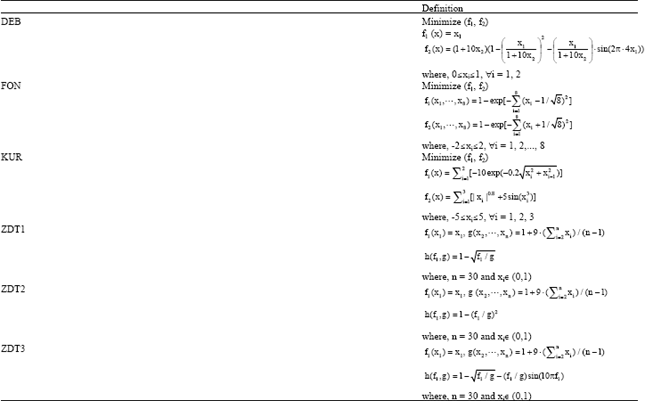 | |
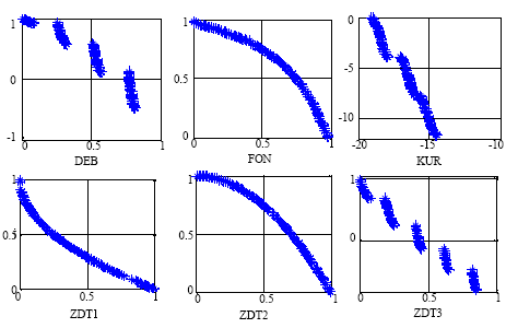 | |
| Fig. 1: | The Pareto optimal fronts of the six test problems |
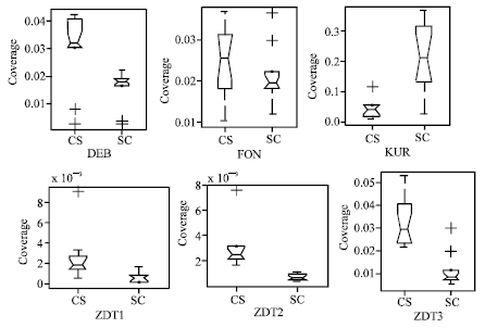 | |
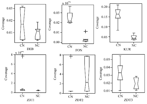
| Fig. 2: | The statistical values of the coverage of the two sets obtained by MCPSO (C) and SPEA2 (S) |
The notched box plots are used to illustrate the results distribution Fig. 2. The notches represent a robust estimate of the uncertainty about the medians for box-to-box comparison. The box has lines at the lower quartile, median and upper quartile values. The whiskers are lines extending from each end of the box to show the extent of the rest of the data. Outliers (the crosses ‘+’) are data with values beyond the ends of the whiskers.
In each plot, the left box represents the distribution of Ic (C, S) and the right box represents Ic (S, C).
Ic (C, S) denotes the ratio of the number of solutions obtained by SPEA2 which are weakly dominated by the solutions obtained by MCPSO to the total number of the solutions obtained by SPEA2 in a single run. Ic (S, C) denotes the ratio of the number of solutions obtained by MCPSO which are weakly dominated by the solutions obtained by SPEA2 to the total number of the solutions obtained by MCPSO in a single run. The comparison between MCPSO and SPEA2 in the coverage of two sets shows that the values of Ic (C, S) and Ic (S, C) for DEB, FON and three ZDT problems are smaller than 0.05. Therefore, only minority solutions are weakly dominated by each other. The box plots of Ic (C, S) are higher than that of Ic (S, C) in DEB, FON and three ZDT problems, while the box plot of Ic (S, C) is higher than that of Ic (C, S) only in KUR.
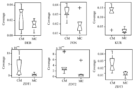 | |
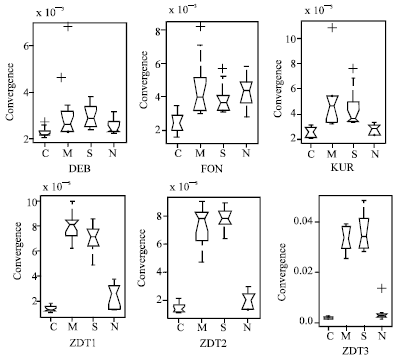
| Fig. 3: | The statistical values of the coverage of the two sets obtained by MCPSO (C) and CMOPSO (M) in solving the six problems |
 | |
| Fig. 4: | The statistical values of the coverage of the two sets obtained by MCPSO (C) and NSGA-II (N) in solving the six problems |
It means MCPSO did better than SPEA2 in DEB, FON and the three ZDT problems while SPEA2 did better than MCPSO in KUR as far as the coverage is concerned (Fig. 3).
In each plot, the left box represents the distribution of Ic (C, M) and the right Ic (M, C).
The comparison between MCPSO and CMOPSO in the coverage of two sets shows that the values of Ic (C, M) are greater than that of Ic (M, C) in all six benchmark problems, it means MCPSO did better than CMOPSO.
The box plots of Ic (C, N) are higher than that of Ic (N, C) in DEB, FON, KUR, ZDT1 and ZDT3 problems, while the box plot of Ic (N, C) is higher than that of Ic (C, N) only in ZDT2. It means MCPSO did better than NSGA-II in DEB, FON, KUR, ZDT1 and ZDT3 problems while NSGA-II did better than MCPSO in ZDT2 problem on the coverage of the two sets.
In each plot of Fig. 4, the left box represents the distribution of Ic (C, N) and the right Ic (N, C).
 | |
| Fig. 5: | The statistical values of the convergence metric obtained by MCPSO (C), CMOPSO (M), SPEA2 (S) and NSGA-II (N) |
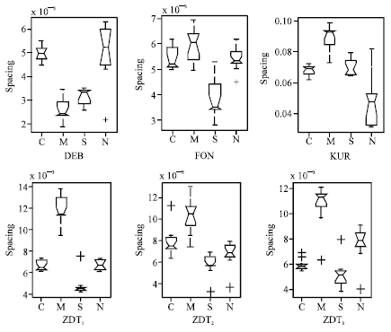 | |
| Fig. 6: | The statistical values of the spacing metric obtained by MCPSO (C), CMOPSO (M), SPEA2 (S) and NSGA-II (N) |
Figure 5 illustrate the convergence metric boxes over 20 independent runs for the six problems. Convergence metric represents the gap between the set of approximate Pareto-optimal solutions and the true Pareto-optimal fronts. It can be concluded that all algorithms can obtain the values less than 0.05 in almost all the 20 independent runs. MCPSO and NSGA-II did better than other two algorithms but MCPSO did best in all four algorithms overall.
Figure 6 illustrate the spacing metric boxes over 20 independent runs for the six problems. The spacing metric means how evenly the solutions are distributed along the discovered front. Figure 6 shows that, for DEB, FON and three ZDT problems, all algorithms obtain the values in 10-3 order of magnitude. MCPSO, SPEA2 and NSGA-II did better than CMOPSO in FON, KUR and three ZDT problems and MCPSO did best in four algorithms.
Overall, it can be concluded that all the four algorithms can approximate the true Pareto optimal fronts for the three low-dimensional problems (DEB, FON and KUR). According to the coverage performance metric, MCPSO did better than SPEA2 in DEB, FON and three ZDT problems. MCPSO did better than CMOPSO in all six test problems. And MCPSO did better than NSGA-II in DEB, FON, KUR, ZDT1 and ZDT3 problems. MCPSO and NSGA-II did better than other two algorithms and MCPSO did best in all four algorithms on the metrics of convergence. MCPSO did best in four algorithms on the metrics of spacing performance.
CONCLUSIONS
In this study, a chaos based PSO strategy is proposed by integrating chaos optimization algorithm and PSO algorithm to solve multi-objective optimization problems. Taking advantages of the ergodic and stochastic properties of chaotic variables, the chaos search is performed in the neighborhoods of particles to exploit the local solution space. The motion of chaotic variables in their ergodic space is used to explore the whole solution space. The coverage of two sets, the convergence metric and spacing metric three performance metrics were used to demonstrate the effectiveness and efficiency of the proposed MCPSO strategy. This study did an attempt for combining promising aspects of different algorithms into an integrated approach that shows good performance on benchmark test problems. This study represented only the first step in the investigation of solving MOP using PSO combined with chaos strategy. Future work will include investigation of the performance of PSO in more complicated higher dimension problems and designing better evolutionary algorithms.
ACKNOWLEDGMENTS
The authors would like to thank the reviewers for their careful reading of this study and for their helpful and constructive comments. This study was supported by the Program for New Century Excellent Talents in University under grant No. NCET-08-0450.
REFERENCES
- Ahmed, B.S. and K.Z. Zamli, 2011. The development of a particle swarm based optimization strategy for pairwise testing. J. Artif. Intell., 4: 156-165.
CrossRefDirect Link - Coello, C.A.C., G.T. Pulido and M.S. Lechuga, 2004. Handling multiple objectives with particle swarm optimization. IEEE Tran. Evol. Comput., 8: 256-279.
CrossRefDirect Link - Cui, Z.H., J.C. Zeng and G.J. Sun, 2006. A fast particle swarm optimization. Int. J. Innovative Comput. Inform. Control, 2: 1365-1380.
Direct Link - Deb, K., A. Pratap, S. Agarwal and T. Meyarivan, 2002. A fast and elitist multiobjective genetic algorithm: NSGA-II. IEEE Trans. Evol. Comput., 6: 182-197.
CrossRefDirect Link - Deb, K., 1999. Multi-objective genetic algorithms: Problem difficulties and construction of test problems. Evol. Comput., 7: 205-230.
CrossRefDirect Link - Fonseca, C.M. and P.J. Fleming, 1995. An overview of evolutionary algorithms in multiobjective optimization. Evol. Comput., 3: 1-16.
CrossRefDirect Link - Fang, X., X. Gao, Z. Yin and Q. Zhao, 2011. An efficient process mining method based on discrete particle swarm optimization. Inform. Technol. J., 10: 1240-1245.
CrossRefDirect Link - Chen, G., 2011. Dynamic optimal power flow in FSWGs integrated power system. Inform. Technol. J., 10: 385-393.
CrossRefDirect Link - Heng, X.C., Z. Qin, X.H. Wang and L.P. Shao, 2006. Research on learning bayesian networks by particle swarm optimization. Inform. Technol. J., 5: 540-545.
CrossRefDirect Link - Lu, H. and X. Chen, 2011. A new particle swarm optimization with a dynamic inertia weight for solving constrained optimization problems. Inform. Technol. J., 10: 1536-1544.
CrossRefDirect Link - Kennedy, J. and R. Eberhart, 1995. Particle swarm optimization. Proc. IEEE Int. Conf. Neural Networks, 4: 1942-1948.
CrossRefDirect Link - Liu, D.S., K.C. Tan, C.K. Goh and W.K. Ho, 2007. A multiobjective memetic algorithm based on particle swarm optimization. IEEE Trans. Syst. Man Cybern., 37: 42-50.
CrossRefDirect Link - Parsopoulos, K.E. and M.N. Vrahatis, 2002. Particle swarm optimization method in multiobjective problems. Proceedings of the ACM Symposium on Applied Computing, March 11-14, 2002, Madrid, Spain, pp: 603-607.
CrossRef - Hernane, S., Y. Hernane and M. Benyettou, 2010. An asynchronous parallel particle swarm optimization algorithm for a scheduling problem. J. Applied Sci., 10: 664-669.
CrossRef - Tong, Z., W. Hongwei and W. Zicai, 1999. Mutative scale chaos optimization algorithm and its application. Control Decision, 14: 285-288.
Direct Link - Yadong, L. and L. Shaoyuan, 2002. A new genetic chaos optimization combination method. Control Theor. Appl., 19: 143-145.
Direct Link - Yang, L.Y., J.Y. Zhang and W.J. Wang, 2009. Selecting and combining classifiers simultaneously with particle swarm optimization. Inform. Technol. J., 8: 241-245.
CrossRefDirect Link - Zitzler, E., L. Thiele, M. Laumanns, C.M. Fonseca and V.G. da Fonseca, 2003. Performance assessment of multiobjective optimizers: An analysis and review. IEEE Trans. Evol. Comput., 7: 117-132.
CrossRef - Zuo, X.Q. and Y.S. Fan, 2006. A Chaos search immune algorithm with its application to neuro-fuzzy controller design. Chaos Solitons Fractals, 30: 94-109.
CrossRefDirect Link