
Zhanmin Wang
Xian University of Technology, China
Duwu Cui
Xian University of Technology, China
Qingzheng Xu
Xian University of Technology, China
Information Technology Journal
Year: 2011 | Volume: 10 | Issue: 11 | Page No.: 2004-2013


ABSTRACT
Prototype reduction algorithms are very useful in the area of nearest neighbor classification and most of them process the given datasets in its entirety. The main disadvantage of them is the excessive computational cost especially when the prototype size is very large. A divide-reduce-coalesce mechanism has been proposed to overcome this shortcoming. But, the final subsets obtained with most of the traditional algorithms in this divide-reduce-coalesce manner are not consistent subsets of original sample set. So, the accuracies of the classifiers obtained in the manner are not been guaranteed too. In this study, we present an artificial endocrine system to reduce useless points in a given training set. The method remains only the points on the boundary between different classes and the amount of reduced rules of the reference set can be revised by the granularity of the lattice. The main advantages of the proposed method are, on the one hand that it is able to condense a given rule set within less time comparing with other traditional algorithms. On the other hand, with the proposed algorithm we can get a consistent subset of the given set in the divide-reduce-coalesce manner. This approach has been tested using 13 different datasets. The experiments show successful results when the size of the given dataset is large.
PDF Abstract XML References Citation
Received: June 28, 2011;
Accepted: August 11, 2011;
Published: September 23, 2011
How to cite this article
Zhanmin Wang, Duwu Cui and Qingzheng Xu, 2011. Artificial Endocrine System and Its Application for Nearest Neighbor Rule Condensation. Information Technology Journal, 10: 2004-2013.
DOI: 10.3923/itj.2011.2004.2013
URL: https://scialert.net/abstract/?doi=itj.2011.2004.2013
DOI: 10.3923/itj.2011.2004.2013
URL: https://scialert.net/abstract/?doi=itj.2011.2004.2013
INTRODUCTION
A classification procedure is a decision-making process in which a pattern xi of unknown class c is assigned to a possible class. To achieve optimal classifier, the procedure usually tries to minimize the classification error (Jiang et al., 2009). Parametric methods assume that the conditional probability density belongs to a certain family of functions and try to get values for the parameters charactering an individual distribution. Nonparametric methods make no assumption on probability distribution and avoid the difficulties involved with the determination of multidimensional conditional probability densities. So a lot of studies are attracted within this area.
Nearest Neighbor (NN) classification is such a nonparametric method to pattern classification. The class of an unknown pattern xi is decided by the similarities between xi and a number of neighbors of it which lie in the neighbor area (Yang et al., 2010). However, for large data sets, the cost to determine the nearest neighbors of a sample point is too expensive. It requires the storage of the complete samples and the computation of N distances if the sample size is N. So, several methods were developed to reduce the size of the sample set while maintaining the advantages of it or to reduce the amount of computation when searching for the nearest neighbor.
The original condensation method, CNN method, is proposed by Hart (1968). The objective of it is to find a consistent reference set. But the output of Hart’s method depends on the order of presentation of the elements in training set X. Dasarathy (1994) represented a Minimal Consistent Set algorithm (MCS) for condensation which does not depend on the order in which the elements of X are processed. Kuncheva and Bezdek (1998) provide a counterexample to Dasarathy’s conjecture that MCS method is truly minimal. Devi and Murty (2002) described a condensation algorithm, called MCNN, in which the prototypes were obtained in an incremental manner. The MCNN algorithm is order independent and many iterative calculations are needed in it to obtain a reduced set. Based on the principle of structural risk minimization, Karacali and Krim (2003) presented a fast reference set thinning method, NNSRM algorithm which was guaranteed to attain zero training error. But the cost is very high and the complexity degree of it is O (|T|3). Mitra et al. (2002) suggested a nonparametric rule reduction algorithm in which multi-scale representative fashion was used to select a subset of a large data set. Chun-Ru et al. (2010) proposed a two-stage condensing algorithm for KNN classifier, in which the noise data were removed firstly and the redundant samples were further eliminated by the definition of Nearest Unlike Neighbor (NUN). Other intelligent algorithms are also used to condensate rules in training set but most of them are suitable for small or medium dataset (Cerveron and Ferri, 2001).
However, to obtain a condensed subset, iterative calculations are always needed for most of traditional algorithms. When the size of the training set is very large, most algorithms are not suitable to condense for the requirement of the storage of the whole training set and the large computation time.
In present study, we present Artificial Endocrine System based nearest neighbor rule condensation method (AES-CNN) to reduce useless points in a given training set. The method remains only the points on the boundary between different classes and the amount of reduced points of the reference set can be revised by the granularity of the lattice. The main advantages of the proposed method are, on the one hand that it is able to condense a given rule set within less time comparing with other traditional algorithms. On the other hand, with the proposed algorithm we can get a consistent subset of the given set in the divide-reduce-coalesce manner.
ARTIFICIAL ENDOCRINE SYSTEM
Based on hormone inspired methodology, Ihara and Mori (1984) and Miyamoto et al. (1984) proposed an Autonomous Decentralized System (ADS), in which a content code communication protocol was used to communicate by a semantics based system. Then, Shen et al. (2002) described a Digital Hormone Model (DHM) in which the advantages of stochastic reasoning, distributed control, self-organization and Turing’s reaction-diffusion model were integrated. The hormone model was also used by Mendao (2007) to coordinate the completion from different tasks by an autonomous robot. In his presentation, tasks were defined as glands and hormones can be released by them at a fixed speed. Once the hormones are greater than a given threshold, they are released and disseminated over the network environment. Walker and Wilson (2008) expanded the model for task assignment to a multiple-autonomous-robots environment. Each task was simply assigned to a robot and each robot can choose a suitable response to the external environment. Now-a-days, artificial endocrine systems are widely used in multiprocessor system control, real time task allocation, human-machine communication and management systems in autonomic networks.
In previous work, Xu and Lei (2011) have proposed a Lattice based Artificial Endocrine System (LAES), in which the system was abstracted as a quintuple model, LAES = (Ld, EC, TC, H, A):
| • | The environment space Ld denotes a bounded area in which all the LAES elements live, die and communicate within it. d is the number of dimensions of the space |
| • | The endocrine cell EC is the fundamental component of the proposed model. Each endocrine cell has a perceiving sensor (AE) and a releaser (BE). The sensor AE can perceive the hormone concentrations of the lattice it lies in. The releaser BE can release a certain quantity of hormone in a discrete manner. In addition, endocrine cells were divided into different kinds. Each kind of endocrine cell can release a special kind of hormone. And every endocrine cell has several different statuses |
| • | The target cell TC is an organ or cell that can accept stimulation from endocrine cells. The receptor AE of TC can perceive the hormone concentrations of the lattice where TC lies. Every target cell has several different statures too |
| • | Hormones are bio-active substances which can be used to adjust the activities of TC and EC. The cumulative hormone concentration at lattice Lxy is equal to the sum of the remaining concentration at time t-1 and newly coming concentration at time t |
| • | Algorithm A is an iterative procedure with which all elements of LAES carry out their assigned task |
NEAREST NEIGHBOR RULE CONDENSATION
The nearest neighbor rule was originally proposed by Cover and Hart (1967). In his subsequent studies Hart (1968) represented a means for decreasing memory and computation requirements.
Assume there are M pattern classes, numbered 1, 2,…, M. Let each pattern be defined in a N-dimensional feature space. Given K training patterns, each of them is a pair (xi,ci), 1≤1≤K and ci ε{1, 2,…, M} denotes the correct pattern class and xi = (x1i, x2i,…, xNi) is the set of feature values of the pattern. Let TNN = {(x1,c1), (x2,c2),…, (xK,cK)} be the nearest neighbor training set. Given an unknown pattern x, the decision rule is to decide x is in class cj if:
| (1) |
where, d (-, -) is some N-dimensional distance metric.
Except the excellent works done by Hart, several other promising methods were proposed. Angiulli (2007) presented a Fast Condensed Nearest Neighbor (FCNN) rule for calculating the consistent subset of a large training set. It is order independent and requires few iteration times to converge. With this algorithm, the selected rules are very close to the decision boundary. Then, Angiuli proposed a distributed version of the FCNN algorithm to reduce the memory consumption and calculation time (Angiulli and Folino, 2007). Based on the definition of chain, Fayed and Atiya (2009) proposed a condensing method TRKNN. The basic idea of the algorithm is to separate the patterns into two different sets, condensed set and removed set, by setting a cutoff value for the chain.
ARTIFICIAL ENDOCRINE SYSTEM FOR NEAREST NEIGHBOR RULE CONDENSATION
The proposed algorithm remains only the points on the boundary between different classes and the amount of reduced rules of the reference set can be revised by the granularity of the lattice. The interior points of a class were seen as unimportant points which should be discarded.
The feature space of a pattern is defined as a discrete lattice environment Ld. Every rule in it is seen as an endocrine cell which has a perceiving sensor and a releaser. The two statuses of an endocrine cell are E0 and E1. In the lattice environment Ld, there is a target cell in every lattice. The there statuses of a target cell are S0, S1 and S2. Each kind of endocrine cell can secrete a special kind of hormone Hci. The only kind of hormone secreted by target cells is H*. The hormone release procedure is a staged process. The target cells were initialized in a sleeping status S0. As long as one kind of hormone was perceived by the target cell, it will get into status S1. If two or more different kinds of hormones were perceived in the same lattice, the target cell will get into status S2. There are two steps in the algorithm:
| Step 1: | All of the rules in training set are seen as endocrine cells and were initialized in status E0. Then, the endocrine cells begin to secrete a fixed mount of hormone to the environment. The hormone will diffuse from high concentration lattices to low ones nearby |
The hormone concentration Hx (I, j,…, n)t+1 of a hormone x at the lattice L (I, j,…, n)t+1 are composed of the remained concentration Hx (I, j,…, n)t at time t and the diffused concentration Δhx (i, j,…, n)t+1 at time t+1:
 |
i, j, …, n are coordinates of the lattice.
Having been stimulated by the hormone, the target cells changed their status according to the kind and concentration of the perceived hormones in a special lattice. When no target cell is still in status S0, the evolutionary process gets into step 2:
| Step 2: | All of the target cells in status S2 secrete hormone H* into the lattice nearby. The concentration of it can be calculated like this: |
where, CHi is the concentration of the hormone Hi and T is the secrete time. After this, the target cells get into status S0.
The hormone H* will diffuse from a lattice L* to a lattice L*’ nearby in which the target cell was still in status S1. After that, the target cell in lattice L* gets in status S0 and the concentration of H* in lattice L*’ will reduce 1 unit. The diffusion process keeps on until the concentration of H* is zero. As long as the endocrine cell perceives the hormone H* in its lattice, the status of it will get into E1. At the end of the diffusion process, all the endocrine cells in status E1 are cells on the boundary of different classes.
Hormone diffusion (single endocrine cell): We can see the diffusion process from Fig. 1 where there is only one endocrine cell in the environment. At time t0, an endocrine cell (red circle) began to secrete hormone Hi. At time t1 (t1 = t0+ΔStstep), the concentration of Hi in the lattice environment was added 1 which was shown with red point.
 | |
| Fig. 1: | Expansion from a single cell |
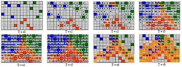 | |
| Fig. 2: | Expansion from multiple endocrine cells |
ΔStstep is the interval of time. At time tk, the diffusion boundary (yi,yj) of hormone Hi secreted by endocrine cell (xi, xj) can be expressed by:
| (2) |
The area of the target cells stimulated by the hormone was expressed by:
| (3) |
When d = 2 (d is the dimension number of the space) and p = 1, the red points shown the area of the target cells in status S1. So, at time t, the area of target cells controlled by an endocrine cell can be expressed by:
| (4) |
Hormone diffusion (multiple endocrine cells): When the number of endocrine cells in the lattice environment is greater than 1, the evolutionary process is shown in Fig. 2, in which 15 endocrine sells (rules), EC1{1}, EC1{2}, EC1{3}, EC1{4}, EC1{5}, EC2{1}, EC2{2}, EC2{3}, EC2{4}, EC2{5}, EC3{1}, EC3{2}, EC3{3}, EC3{4} and EC3{5} were set in the lattice. They belong to three different classes: 1, 2 and 3 (indicated by blue, red and green squares). In each lattice, there lives a target cell. At time t0, all of the target cells (expressed by empty squares) are in status S0 and all of the endocrine cells (expressed by color square) are in status E0. At time t1, endocrine cells secreted their hormones. The concentration of hormone in a lattice was expressed by a color point. When the target cell was stimulated by a hormone, they turned into status S1. At time t2, 6 target cells perceived two or more kinds of hormones in their lattices and turned into status S2 (expressed by orange squares). As the time goes by, more and more hormones were spread out. At time t5, no target cell was in status S0. The first evolutionary stage ended.
In the second stage, all the target cells in status S2 secreted the hormone H* (yellow points) and then turn into status S0. The hormone H* spread out in the environment from high concentration lattices to the low one. Each time it takes place, the value of the concentration was subtracted 1. When the concentration of H* was reduced to zero, at time t9, the evolutionary process stopped. The endocrine cells who perceives hormone H* in their lattices turned into status E1. And the endocrine cells in status E1 are cells we searched.
ALGORITHM ANALYSIS
Consistency analysis: Let TNN = {(x1, c1), (x2, c2), …, (xK, cK)} be the set of training samples, ci (ci ε {1, 2,…, M}) be the class label of a sample (xi, ci), xi = (x1i, x2i,…, xNi) be the feature set of the sample.
Definition 1 (Sample distance): The sample distance d ((xi, ci), (xj, cj)) between two samples (xi, ci) and (xj, cj) in N-dimension space is:
| (5) |
Definition 2 (Consistent subset): A consistent subset TCNN of training sample set TNN is a subset of TNN that could classify all the patterns in TNN correctly.
Definition 3 (Minimal consistent subset): The minimal consistent subset TMCNN is the smallest and most efficient subset of TNN that could properly classify every pattern in TNN.
Theorem 1: The subset TAES-CNN of a given sample set TNN, obtained by algorithm AES-CNN, is a consistent subset of TNN.
Proof: Let TNN1 be the set of endocrine cells which are in E1 status at the end of the second stage. Let TNN2 be the set of endocrine cells which are in E0 status at the end of the second stage.
According to algorithm AES-CNN, the training sample set TNN is composed of TNN1 and TNN2:
 |
Let (xj, cj) be a cell in TNN2. Let (x*, c*) be the nearest cell of cell (xj ,cj) and the two cells have the same class label. Let (x&,c&) be the nearest cell of cell (xj,cj) and the two cells have the different class label. Thus:
If we want to show that TNN1 is a consistent subset of TNN, the only task for us is to show that for every cell (xj,cj) in TNN2, the assertion below is true:
Assume:
Then, according to rules in step 1, there will be a target cell TCk which was stimulated by the two kind of hormones released by cell (x&, c&) and cell (xj, cj).
Thus, in the second stage, the TCk will release hormone H*. And then, having been stimulated by hormone H*, the cell (xj, cj) will come into state S0. So, the cell (xj, cj) should belong to TNN1.
However, it is a contradictious assertion against the assumption (xj,cj)εTNN2.
So, we can get d ((x*, c*), ( xj, cj))≤d ((x&, c&), (xj, cj)).
Complexity analysis: Complexity of an algorithm refers to the amount of time and space required to execute the algorithm in the worst case. AES-CNN algorithm is a parallel algorithm. If we implement it in a series manner, the time needed to execute it comprises with two main parts:
| • | In the first stage: the N coordinates of the N-dimension space are divided into n1,n2,…nN uniform lattices. The endocrine cells (sample rules) were placed in the lattice environment and released a certain amount of hormones at every discrete time. In the worst cases, these can be performed in O (Nxn1xn2x,…xnNxn*) time. n* is the maximal elements in the set {n1,n2,…nN} |
| • | In the second stage: the target cells were stimulated and released hormone H*. The concentration of H* in a lattice was subtracted 1 every discrete time. These can be performed in O (Nxn1xn2x,…xnNxn*) time |
By summing up the computational time required for each of the two stages, it is possible to determine the total computational time of the algorithm. The computational time of the whole process is given by:
| (6) |
It is clear that the computational time of the algorithm is determined mainly by the number of the dimension, the numbers of the discrete lattices in each coordinates axis.
The memory required to run the algorithm is proportional to the number of samples K, dimensions N and the number of discrete lattices.
EXPERIMENTAL RESULTS
The experiments were conducted on a 3.0 GHz Pentium4 with 1.0 GB of memory running Microsoft Windows XP. All code was compiled using Microsoft Visual C++6.0. The datasets used in the experiment are obtained from the UCI Machine Learning Repository (Newman et al., 1998).
Data preprocessing: In AES-CNN algorithm, the lattice granularity is an important parameter. Too small size of it will lead to a slow implementation. So, in order to speed up the implementation process, we preprocess the training set like this:
Let Z (I, j, …, n) be the location of an endocrine cell and i, j,…, n are coordinates. In general, the values of them are always real number. In order to assign a suitable value for each of them, we give several preprocessing operations:
| • | Rank the endocrine cells according to their coordinate i, the former is the smaller. And then, assign new value for each of this coordinate i like this: 1, 2, …, M |
| • | Rank the endocrine cells according to their coordinate j, …, n and assign new value for each of the coordinate just like it in (step 1) |
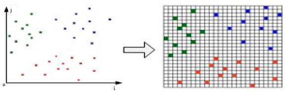 | |
| Fig. 3: | Data preprocessing |
| Table 1: | Different granularities (Iris) |
 | |
After doing so, we can see the endocrine cells in the lattice environment from Fig. 3.
Lattice granularity: Here, the data set used is Iris. There are 150 instances, 4 condition attributes and 1 class attribute in it. We divided the data set into two parts: training set (120 instances) and test set (30 instances). With the proposed AES-CNN algorithm, we delete some rules in training set and obtained the consistent subset of it. From Table 1, we can see that the numbers of the deleted rules and remained rules, the accuracy of the classifier built by the remained rules and the time needed are listed in column 5, 6, 7 and 8. We divided the 4 condition attributes with different grain sizes (we can see it from column 1). That leads to different number of lattices in the artificial endocrine environment.
From Table 1, we can see that as the increasing of the grain size of the lattice, the number of the lattices becomes smaller and the running time of the algorithm gets faster. However, the accuracy of the algorithm becomes more less.
When the value of column 5-C is 0, we can see that the accuracy of the record 1-3 keep unchanged, although the grain size was enlarged. But for record 4-5, the accuracy of it declined. The reason is that the decline of the accuracy of the algorithm mainly decided by the grain size of the lattice. When different classes of cells were swallowed in the initial step, the algorithm can not find the right boundary in the evolution stage. For example, in record 4 and 5, the numbers of the swallowed rules of different class labels were 7 and 38. So, the unsuitable grain size of the lattice will lead to incorporation of the rules in different class. As a result, the classification accuracy will decline. However, after preprocessing, the algorithm will find a classifier faster on the case of similar accuracy.
Different instance size: Here, the data sets used are Car and Transfusion. There are 1728 records and 4 class labels in dataset Car and 748 records and 2 class labels in dataset Transfusion. We randomly divided the two data sets into two parts: one for training (1530, 592 instances), one for test (198, 156 instances). Then, we choose rules from training set to build 9 different sub-training sets. The instance numbers of the sub-training sets in Car are 170, 340, … , 1530, in Transfusion are 74, 148,…,592.
From Fig. 4 we can see that with the increasing of the number of the training instances, the accuracies of the two algorithms AES-CNN and algorithm CNN [3] improve simultaneously. However, when the number of the training instances is small, the accuracy of algorithm CNN is greater than AES-CNN. When the number of the training instances gets large, the accuracy of the two algorithms are almost the same. It is because that the remained rules obtained by AES-CNN are boundary cells but by CNN, they are cells selected randomly. When the boundaries between different classes are complex, more boundary cells were remained and the accuracy of the algorithm AES-CNN is low and unstable. We can see it from Fig. 4. For dataset Car, the accuracy of AES-CNN is lower than CNN and the number of the rules remained in AES-CNN is larger than it in CNN.
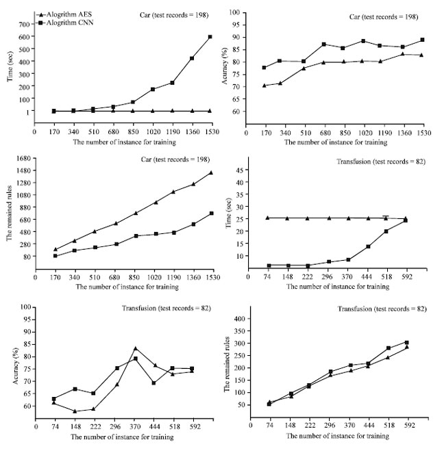 | |
| Fig. 4: | Different sizes of training set |
However, for dataset Transfusion, the accuracies of the two algorithms and the remained rules of them are very similar. Why? The reason is that for dataset Transfusion, the numbers of the feature attributes and classes are small. The boundary of the dataset is very simple. So, the boundaries between different class cells can be recorded by fewer boundary cells.
Comparing with the accuracy and the number of remained rules in the two algorithms, the runtime of the two algorithms are so different. For both of them, with the increasing of the training instances, the time cost by CNN increased quickly. But the time cost by AES-CNN is fixed. The difference between the two datasets is that, for Car, the runtime of AES-CNN is less than CNN. For Transfusion, the runtime of AES-CNN is more than CNN.
We can find the reason from formula (6) which shows that the computational time of CNN is O(K!) while for AES-CNN, the time is O(2xNxn1xn2x,…xnNxn*). For a given dataset, when the dimensions and grain size of lattice are fixed, the running time of algorithm AES-CNN is fixed. When the number of the records is small and the attributes of it is large, the efficiency of algorithm CNN will greater than AES-CNN. Otherwise, the efficiency of algorithm AES-CNN will greater than CNN.
| Table 2: | Performance results on different datasets |
 | |
| Table 3: | Consistency comparison-3 |
 | |
Comparisons with different datasets: In Table 2, we compared the proposed AES-CNN algorithm with CNN, TRKNN and FCNN algorithms on 13 datasets coming from UCI Machine Learning Repository. Each dataset was divided into two parts: training set and test set. The size of the train set, the percent of the accuracy and storage of the classifier (comparing with no condensate one) and the runtime of the algorithm are shown in Table 2.
As can be seen, as the size of the training set getting larger, AES-CNN showed more feasible on runtime. For example, on dataset Car, the runtime of AES-CNN is less than 1 sec. However, for CNN, it is 430 sec. But the efficiency of AES-CNN is constrained by the grain size of the lattice. When there are too many lattices in the AES circumstance, AES-CNN will cost more runtime. For example, on dataset Tae, the runtime of AES-CNN is 42 seconds which is much longer than that of algorithm CNN.
In general, the accuracy of the classifier obtained by algorithm AES-CNN is higher than others. But the difference is not very obvious. The numbers of the rules used to build the classifier are very different. For AES-CNN, more remained rules were left. The reason of that is the nature of the algorithm AES-CNN is to find the boundary cells, the number of which is generally larger than the number of the remained rules gotten by CNN or other algorithms when the distributions of different classes in a given dataset are very complex.
With the comparison above we can find that the algorithm AES-CNN is more suitable for the case where the size of the dataset is very large. When the boundary between different classes is very complex, the size of the condensate subset gotten by AES-CNN is larger than that gotten by other algorithms. On the contrary, the size is less than others.
Consistency comparison (divide-reduce-coalesce manner): Here, we check the consistency of the proposed algorithm with divide-reduce-coalesce manner. The two datasets used in this section are Car and Transfusion. In step 1, we randomly split an original set A0 into four subsets, A1, A2, A3 and A4. Then, we condensed the four subsets, respectively with different algorithms and obtained four sets, A1’, A2’, A3’ and A4’. In step2, we obtained set B1 by integrating the two sets A1’ and A2’ and obtained set B2 by integrating A3’ and A4’. In step3, we condensed the two sets B1, B2 and obtained two subsets B1’ and B2’. Finally, we integrate the sets B1’, B2’ and condensed them to get the terminal set C. The original set A0 was seen as the test set.
From Table 3, we can see that after the divide-reduce-coalesce condensation, all of the final four subsets gotten by four different algorithms are not consistent sets of the original given set A0. However, the accuracy of algorithm AES-CNN is far higher than algorithms CNN, TRKNN and FCNN. And the runtime of algorithm AES-CNN in such a manner is also superior to other algorithms.
The reason why the subset C obtained by algorithm AES-CNN is not a consistent subset of A0 lies in the manner of data preprocessing and the manner of distance calculation. The distances between different points, calculated with discrete coordinates, are not accurate ones. Even so, from the experiments we can see that the AES-CNN algorithm is more suitable for divide-reduce-coalesce learning than other algorithms.
DISCUSSION AND CONCLUSION
The algorithm presented in this study is an artificial endocrine system based nearest neighbor rules condensation approach. The main advantages of this method are, on the one hand that it is able to condense a given rule set within less time when the number of the rules in a given rule set is very large. On the other hand, with the algorithm, we can get a consistent reference set of the given set in an iterative or accumulated manner.
To achieve this, an artificial endocrine model was developed so as to a parallel complementation of the condensation process. Previous works pay more attentions to the accuracy of the classifier built by the remained rules. But the implement time increases very quickly as the rule number becomes more and more large. However, in this study we pay more attentions to the reduction of the runtime and the capability of the accumulated running. The method remains only the points on the boundary between different classes. The algorithm can guarantee little resubstitution error and at the same time, the generalization capability of the nearest prototype classifier is considered.
ACKNOWLEDGMENT
We are grateful to the anonymous referees for their invaluable suggestions to improve the study. This work was supported by the National Natural Science Foundation of China (60873035).
REFERENCES
- Jiang, L., H. Zhang and Z. Cai, 2009. A novel bayes model: Hidden naive bayes. IEEE Trans. Knowledge Data Eng., 21: 1361-1371.
CrossRef - Yang, J.M., P.T. Yu and B.C. Kuo, 2010. A nonparametric feature extraction and its application to nearest neighbor classification for hyperspectral image data. IEEE Trans. Geosci. Remote Sensing, 48: 1279-1293.
CrossRef - Hart, P., 1968. The condensed nearest neighbor rule (Corresp.). IEEE Trans. Inform. Theory, 14: 515-516.
CrossRef - Dasarathy, B.V., 1994. Minimal consistent set (MCS) identification for optimal nearest neighbor decision systems design. IEEE Trans. Syst. Man Cybernet, 24: 511-517.
CrossRef - Devi, V.S. and M.N. Murty, 2002. An incremental prototype set building technique. Pattern Recognition, 35: 505-513.
CrossRef - Karacali, B. and H. Krim, 2003. Fast minimization of structural risk by nearest neighbor rule. IEEE Trans. Neural Networks, 14: 127-134.
CrossRef - Mitra, P., C.A. Murthy and S.K. Pal, 2002. Density-based multiscale data condensation. IEEE Trans. Pattern Anal. Machine Intell., 24: 734-747.
CrossRef - Chun-Ru, D., P.P.K. Chan, W.W.Y. Ng and D.S. Yeung, 2010. 2-Stage instance selection algorithm for KNN based on Nearest Unlike Neighbors. Proceedings of the International Conference on Machine Learning and Cybernetics, July 11-14, Qingdao, pp: 134-140.
CrossRef - Cerveron, V. and F.J. Ferri, 2001. Another move toward the minimum consistent subset: A tabu search approach to the condensed nearest neighbor rule. IEEE Trans. Syst. Man Cybernetics Part B, 31: 408-413.
CrossRef - Ihara, H. and K. Mori, 1984. Autonomous decentralized computer control systems. IEEE Comput., 17: 57-66.
CrossRef - Miyamoto, S., K. Mori, H. Ihara, H. Matsumaru and H. Ohshima, 1984. Autonomous decentralized control and its application to the rapid transit system. Int. J. Comput. Ind., 5: 115-124.
CrossRef - Shen, W.M., B. Salemi and P. Will, 2002. Hormone-inspired adaptive communication and distributed control for CONRO self-reconfigurable robots. IEEE Trans. Robotics Automation, 18: 700-712.
CrossRef - Walker, J. and M. Wilson, 2008. A performance sensitive hormone-inspired system for task distribution amongst evolving robots. Proceedings of the IEEE/RSJ International Conference on Intelligent Robots and Systems, Sept. 22-26, New York, pp: 1293-1298.
CrossRef - Xu, Q.Z. and W. Lei, 2011. Lattice-based artificial endocrine system model and its application in robotic swarms. Sci. China Inform. Sci., 54: 795-811.
CrossRef - Cover, T. and P. Hart, 1967. Nearest neighbor pattern classification. IEEE Trans. Inform. Theory, 13: 21-27.
CrossRefDirect Link - Angiulli, F., 2007. Condensed nearest neighbor data domain description. IEEE Trans. Pattern Anal. Machine Intell., 29: 1746-1758.
CrossRef - Angiulli, F. and G. Folino, 2007. Distributed nearest neighbor-based condensation of very large data sets. IEEE Trans. Knowledge Data Eng., 19: 1593-1606.
CrossRef - Fayed, H.A. and A.F. Atiya, 2009. A novel template reduction approach for the k-nearest neighbor method. IEEE Trans. Neural Networks, 20: 890-896.
CrossRef - Kuncheva, L.I. and J.C. Bezdek, 1998. Nearst prototype classification: Clustering, genetic algorithms, or random search?. IEEE Trans. Syst., Man, Cyber. Part C, 28: 160-164.
CrossRefDirect Link