
Cheng Ma
Control and Simulation Center, Harbin Institute of Technology, Harbin China
Ye San
Control and Simulation Center, Harbin Institute of Technology, Harbin China
Yi Zhu
Control and Simulation Center, Harbin Institute of Technology, Harbin China
Information Technology Journal
Year: 2013 | Volume: 12 | Issue: 4 | Page No.: 847-851


ABSTRACT
The truncated particle filter was proposed based on the analysis of residual particle filter and regularized particle filter. The main idea of the truncated particle filter was to draw the new particles from the resampling area of the particles with large weights, rather than point-wise determine the repetition number of each particle. The effective resampling areas were established by these particles whose weights were larger than the truncated value. The uniform kernel was used to draw new particles from these areas. This method combined the information contained in the prior transformation function and the likelihood function, meanwhile increased the particle diversity. The simulation results showed that the truncated particle filter reduces the computational complexity, meanwhile maintains the same estimation accuracy as the common resampling algorithms. Furthermore, this new algorithm greatly shortened the estimated time and improves the stability of the estimates.
PDF Abstract XML References Citation
Received: August 20, 2012;
Accepted: December 04, 2012;
Published: January 22, 2013
How to cite this article
Cheng Ma, Ye San and Yi Zhu, 2013. A Kind of Truncated Particle Filter. Information Technology Journal, 12: 847-851.
DOI: 10.3923/itj.2013.847.851
URL: https://scialert.net/abstract/?doi=itj.2013.847.851
DOI: 10.3923/itj.2013.847.851
URL: https://scialert.net/abstract/?doi=itj.2013.847.851
INTRODUCTION
As the Bayesian filtering approach, the particle filter which is based on sequential Monte Carlo sampling can effectively deal with the non-linear and non-Gaussian problems. In recent years, this method has been applied in many areas, such as digital communications, financial data analysis, image processing, adaptive estimation, speech signal processing, machine learning and et al. The Sequential Importance Sampling (SIS) algorithm was proposed in 1950s which is viewed as the prototype of the particle filter. Gordon et al. (1993) proposed the Sampling Importance Resampling (SIR) method in recursive Bayesian filter (Gordon et al., 1993). And a lot of improvements are proposed after that, such as Gaussian/Gaussian sum particle filter (Kotecha and Djuric, 2003a, b), unscented particle filter (Cheng and Bondon, 2008), regularized particle filter (Musso et al., 2001). A few tutorials have already been published on the subject (Arulampalam et al., 2002; Cappe et al., 2007; Arnaud and Johansen, 2011).
The resampling schedule is a very intuitive idea but plays an important role in the particle filter. Currently, in literature quite a few different resampling methods can be found. To summarize, the three most popular algorithms of them are multinomial resampling, residual resampling, stratified resampling/systematic resampling (Arnaud and Johansen, 2011). The basic idea of these resampling schedules is to replicate the particles with large weights, meanwhile removing the ones with small weights. As a result, the number of the particles is the same in every generation. Hol et al. (2006) analyzed these algorithms in term of the resampling quality and computational complexity.
The resampling schedule mentioned above relieves the particle degeneracy but also introduces the limitation of the calculation speed of the particle filter. This means that the new particle set is established after the repetition number of each particle in the original set is calculated. On the other hand, Gordon et al. (1993) and Musso et al. (2001) point out that the particle system will concentrate in areas of interest of the state space if the more likely particles are selected. So if these areas were established firstly, then draw the new particles from the areas, we could get the new particle set. So this paper study the areas of interest of the state space and ‘resample’ the new particles from these areas.
PARTICLE FILTERS
Dynamic state-space model: The general nonlinear, non-Gaussian dynamic state-space model can be expressed as follows:
| (1) |
| (2) |
where, xk denotes the state of the system and follows a Markov process, yk is the output observation, vk and nk are i.i.d. process noise and observation noise, respectively, fk represent the deterministic process and hk represent the measurement models. The initial distribution (at k = 0) is donated by p(x0) in order to complete the specification of the model.
Generic particle filer: The generic particle filter consists of Sequential Importance Sampling (SIS) and resampling schedule. This section begins with the SIS method, then describes the residual resampling and the regularized resampling which are mainly concerned in this study.
Sequential importance sampling: Given all the available information, the posterior probability density function of the current states x0:k can be approximated as:
| (3) |
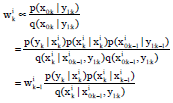
where, δ() is the Dirac delta measure, {xi0:k, i = 1, …, N} is a set of support particles with associated weights {wik, i = 1, …, N}. And the weights are normalized such that ![]() . As N→∞, the discrete weighted approximation will approach the true posterior density p(x0:k|y1:k). But drawing from p(x0:k|y1:k) directly is usually different. So the particles are actually drawn from a proposal distribution q() which is called an important density. And the so-called importance weights are defined as:
. As N→∞, the discrete weighted approximation will approach the true posterior density p(x0:k|y1:k). But drawing from p(x0:k|y1:k) directly is usually different. So the particles are actually drawn from a proposal distribution q() which is called an important density. And the so-called importance weights are defined as:
 | (4) |
A simple but efficient choice of the important density is the priori probability density:
| (5) |
The new estimate of the p(x0;k|x1:k) is given by:
| (6) |
Where:
| (7) |
Resampling: To avoid the degeneracy of the SIS algorithm, a resampling schedule is introduced in order to eliminate samples with low importance weights and replicate samples with high importance weights. As mentioned before, there are three of the most commonly used resampling approaches. In this paper, we will describe some details of residual resampling.
The new particle set consists of the main particle set and the residual particle set in the residual particle filter. And the main particle set is determined by the integer component and the residual particle set is achieved through the multinomial resampling. A pseudo-code description of the residual resampling is given by algorithm 1:
| Algorithm 1: | Residual resampling |
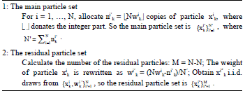 | |
Residual resampling considers the expected number of replications of each particle and deterministically replicates some of the particles, then the non-integer (residual) components of Nwik are treated. So the degree of randomness introduced by the resampling procedure is reduced and the residual resampling has smaller Monte Carlo variance (Liu and Chen, 1998).
Regularized particle filter (RPF): The RPF is identical to the generic particle filter, except for the resampling schedule. In the generic particle filter, the resampling produces a new particle set where several particles may have the same location in the state space. The situation will be worse when the system noise is small or nonexistent and the particle system may rapidly collapse to a single value. So the regularized particle filter was proposed to increase the diversity of the filter.
The basic idea of RPF is that the samples are draw from a continuous distribution rather than a discrete one in generic particle filter. The RPF resampling from a continuous approximation of the posterior density which is obtained by using the kernel density estimation method:
| (8) |
where, Kh = (1/hn) K(x/h) is a rescaled Kernel density, h>0 is the kernel bandwidth, ni is the dimension of the state vector. The kernel density is a symmetric probability density function.
The kernel K() and the bandwidth h are chosen to minimize the mean integrated square error. In the special case of all the samples having the same weight and the underlying density is Gaussian with unit covariance matrix, the optimal choice of the kernel is the Epanechnikov kernel.
Truncated particle filters: As described above, the new particle set consists of the main particle set and the residual particle set in the residual particle filter. The main particle set contains those particles with larger weights and the weights of those particles are actually larger than 1/N. If the threshold is smaller, then the more particles will fall in the main particle set. So the new main particle set is:
| (9) |
where, kt is the truncated value.
The main particle set will be a special subset of the original particle set which only contains a few of those particles but the sum of the weights will approach 1 as kt increases. In the particle filter, the resampling schedule will multiply the particles with the larger weights and discard those with smaller weights. It is easy shown that almost all of the multiplied particles will be in the main particle set if kt is larger enough. These particles in the main particle set will be ‘effective particles’. The main purpose of establishing the residual particle set is to ensure the same number of particles and increase the particle diversity.
In particle system, the intuition is that the more particles selected from the areas of interest of the state space, the better estimation of the posterior probability. Based on the information at hand, the spatial extent of the main particle set is equivalent to these areas which could be established by inequality Eq. 9.
After these areas are established, the regularized resampling could be applied on them. As mentioned above, the normal choice is the Epanechnikov or Gaussian kernel. But in this paper, the uniform kernel is used. There are three reasons for doing this. Firstly, the uniform kernel is the simplest one of the kernel functions which are commonly used. Secondly, the particle filter deal with a cloud of particles, not single one. So the drawing could be applied almost simultaneity. Last but not least, a large number of particles could reduce the errors due to the different regularizations. For example, in the case where the process noise is small, the particle system may rapidly collapse to a single particle (Gordon et al., 1993). The particle filter could draw the new particles from the areas around the single one by the regularization. Then the errors due to the different regularizations might be smaller as the number of the particles increases. So the truncated particle filter is proposed in this study.
A pseudo-code description of the truncated particle filter is then given by algorithm 2.
| Algorithm 2 | |
 | |
The systematic diagram for truncated particle filter is shown in Fig. 1. The new algorithm is equivalent to the SIS algorithm with a band-pass filter. The likelihood function is used as the filter which removes the particles with the low weights while retaining the ones with large weights.
After introducing the proposed algorithm, we will discuss the choice of some parameters:
| • | The range of the truncated value kt. This value could be constant or changed with the sum of the weights in the main particle set. Firstly, as a constant, kt is equal to 1 in the residual particle filter. As the truncated value decreases, there are more particles in the main set. The TPF is equal to the SIS algorithm when the whole particles are in the main set which means that kt is very large. So we recommend the range of the truncated value is [2,4]. Otherwise, this value could be set as the sum of the weights in the main particle set is larger than a special value, such as 0.98 |
| • | The disturbance of the single particle. There is common phenomenon that the particle system might concentrate on a single point of the state space and this point is an ‘isolated point’. In TPF, this means that xmin is equal to xmax. Gordon et al. (1993) point out that the ‘brute force’ approaches could overcome this difficulty by using the disturbance. The solution is replicating this particle as the normal resampling schedule or resampling randomly around this particle in very small areas |
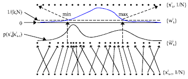 | |
| Fig. 1: | Systematic diagram for truncated particle filtering |
SIMULATION
Here, we consider a Univariate Non-stationary Growth Model (UNGM) and the process model and measurement model of the simulated objects are given as follows:
| (10) |
where, uk and vk are zero mean Gaussian random variable with variances Qk and Rk, respectively. Given the process noise variance Qk = 10 and the measurement noise variance Rk = 1, the particle number is N = 100. And the initial state was taken to be x0 = 0.1 with variance q = 5. This system has been analyzed in many publications.
In this study, the estimation and prediction of the SIS, Residual Particle Filter (RrPF), System Particle Filter (SrPF), Multinomial resampling Particle Filter (MrPF) and Truncated Particle Filter (TPF) are compared with the root mean square error which is defined as:
| (11) |
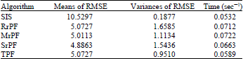
After 500 times of Monte-Carlo simulation, the average result is given in Fig. 2 and Table 1.
According to the simulation results and figures, the following information can be easily obtained:
| • | Estimation result: The state estimation results of the multinomial resampling particle filter, the residual resampling particle filter, the system resampling particle filter and the truncated particle filter are very close. But the variance of the RMSE of the truncated particle filter is less than the other algorithms. This means that the new proposed algorithm is more stable than the other resampling schedules |
| • | Running time: The running time of the truncated particle filter is much less than the other three resampling algorithms, even close to the SIS resampling algorithm. The reason is that the new algorithm focuses to obtain the effective areas of particles, rather than to establish particles point by point. The other three resampling algorithm consider the repetitions of each particle, thereby increasing the running time |
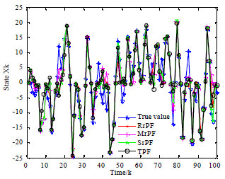 | |
| Fig. 2: | True values of the state, estimated values of various algorithms |
| Table 1: | Comparison between average RMSEs and runtime of various algorithms |
 | |
CONCLUSION
Firstly, the residual particle filter and regularized particle filter are analyzed and then a kind of truncated particle filter is proposed based these particle filters. The new algorithm establishes the areas of interest of the state space only by using the truncated value and resamples the new particles uniformly from these areas, so the computation efficiency is improved. Moreover, the filtering accuracy is still as low as the popular resampling schedule. The next phase of the study is to improve filtering accuracy while reducing the computational time.
ACKNOWLEDGMENT
This study is supported by the National Natural Science Foundation of China under Grant No. 61074127.
REFERENCES
- Gordon, N.J., D.J. Salmond and A.F.M. Smith, 1993. Novel approach to nonlinear/non-Gaussian Bayesian state estimation. IEE Proc. F Radar Signal Process., 140: 107-113.
CrossRef - Arulampalam, M.S., S. Maskell, N. Gordon and T. Clapp, 2002. A tutorial on particle filters for online nonlinear/non-Gaussian Bayesian tracking. IEEE Trans. Signal Processing, 50: 174-188.
CrossRef - Cappe, O., S.J. Godsill and E. Moulines, 2007. An overview of existing methods and recent advances in sequential Monte Carlo. Proc. IEEE., 95: 899-924.
CrossRefDirect Link - Arnaud, D. and A.M. Johansen, 2011. A Tutorial on Particle Filtering and Smoothing: Fifteen years later. In: Handbook of Nonlinear Filtering, Crisan, D. and B. Rozovskii (Eds.). Oxford University Press, New York, pp: 656-704.
Direct Link - Hol, J.D., T.B. Schon and F. Gustafsson, 2006. On resampling algorithms for particle filters. Proceedings of the IEEE Nonlinear Statistical Signal Processing Workshop, September 13-15, 2006, Cambridge, UK, pp: 79-82.
CrossRefDirect Link - Cheng, Q. and P. Bondon, 2008. A new unscented particle filter. Proceedings of the IEEE International Conference on Acoustics, Speech and Signal Processing, March 30-April 4, 2008, Caesars Palace, Las Vegas, Nevada, USA., pp: 3417-3420.
CrossRef - Kotecha, J.H. and P.M. Djuric, 2003. Gaussian particle filtering. IEEE Trans. Signal Proc., 51: 2592-2601.
CrossRefDirect Link - Kotecha, J.H. and P.M. Djuric, 2003. Gaussian sum particle filtering. IEEE Trans. Signal Proc., 51: 2602-2612.
CrossRefDirect Link - Liu, J.S. and R. Chen, 1998. Sequential monte carlo methods for dynamic systems. J. Am. Statisti-cal Assoc., 93: 1032-1044.
Direct Link