
Li Zhang
College of Science, Yanshan University, Qinhuangdao, Hebei, 066004, China
Xiangdong Song
College of Science, Yanshan University, Qinhuangdao, Hebei, 066004, China
Information Technology Journal
Year: 2014 | Volume: 13 | Issue: 14 | Page No.: 2369-2373


ABSTRACT
In order to reduce the number of observations to signal when the shifts occurs in the process, this study proposed the Exponentially Weighted Moving Average (EWMA) median control charts with Variable Sampling Size (VSS). Give the distribution function of the median value assume that the distribution of observations from a process is normally distributed. Then using the Markov chain method to establish a model to calculate the average number of observations to signal (ANOS) of median control chart. Finally, compare the ANOS of the new model with that of the conventional fixed sampling size EWMA control chart and VSS EWMA mean control chart. The data showed that, the designed new model can effectively reduce the ANOS when the process is out of control. That is to say, the new model effectively improves the efficiency of the monitoring process, shifts can be discovered in a shorter period of time which make a great significance to the actual production.
PDF Abstract XML References Citation
Received: March 14, 2014;
Accepted: May 19, 2014;
Published: June 07, 2014
How to cite this article
Li Zhang and Xiangdong Song, 2014. EWMA Median Control Chart with Variable Sampling Size. Information Technology Journal, 13: 2369-2373.
DOI: 10.3923/itj.2014.2369.2373
URL: https://scialert.net/abstract/?doi=itj.2014.2369.2373
DOI: 10.3923/itj.2014.2369.2373
URL: https://scialert.net/abstract/?doi=itj.2014.2369.2373
INTRODUCTION
Statistical process control is an effective method for improving product quality and saving firm’s productivity (Baxley, 1995; Chou et al., 2006). The major tool of statistical process control is the control chart. The Exponentially Weighted Moving Average (EWMA) charts were first introduced by Roberts (1959) and have been widely used in statistical process control for monitoring process shifts (Chang and Bai, 2001; Crowder, 1989). When the process shifts are small, they can find promptly (Costa, 1997). To improve the inspection efficiency of control charts, VSS Shewhart control chart was firstly proposed by Prabhu et al. (1993, 1994) and Costa (1994) respectively, Reynolds and Arnold (2001), Reynolds (1996), Saccucci and Lucas (1990) proposed the EWMA control charts with Variable Sampling Interval (VSI) and so far, the research achievements about VSS control-chart is not so abundant than VSI control-chart (Ji et al., 2006; Wang, 2002). Although, there is a part of literature focused on VSS control chart, very little work has been done on the median design of the VSS control chart (Zhang, 2000).
DESCRIPTION OF THE VSS EWMA MEDIAN CONTROL CHART
Assume that the distribution of observations X from a process is normally distributed and has a mean of μ and a known variance of σ. Then the i-th sample statistic of EWMA chart is:
| (1) |
where, λ is the exponential weight constant, Z0 is the starting value and is often taken to be the process target value and the sequentially recorded observations Xi can either be individually observed values from the process or sample averages obtained from rational subgroups. Here, we took Xi as sample median obtained from rational subgroups, then the i-th sample statistic of EWMA chart is:
| (2) |
When i is zero, Z0 = μ0, When the process is in control, then we have:
| (3) |
| (4) |
So:
| (5) |
| (6) |
where, D(![]() ) is the variance of distribution function of the median and σZ is the standard deviation.
) is the variance of distribution function of the median and σZ is the standard deviation.
Then the upper and lower control limits for the VSS EWMA chart can be written as:
| (7) |
| (8) |
Generally we adopt its asymptotic form:
| (9) |
| (10) |
where, r is the control limit coefficient of the VSS EWMA chart. The upper and lower warning limits for the EWMA chart are:
| (11) |
| (12) |
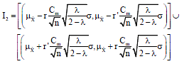
where, r' (0<r'<r) is the warning limit coefficient of the VSS EWMA chart. Then we can get the two regions of the chart.
Where:
| (13) |
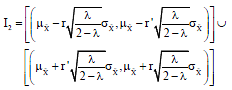 | (14) |
When designing the control chart with variable sampling size, we choose two sampling size n1 and n2, moreover n2>n>n1. Divide the control charts into center region and alert region. The I1 is the center region and the alert region is I2. If the sample statistic falls in the safe region I1, then take the next sample using n1. If the sample statistic falls in the warning region I2, then take the next sample using n2. If the sample statistic falls outside the control limits, then give a signal and search for the cause.
DISTRIBUTION FUNCTION OF THE MEDIAN
When X~N(μ, σ2), n = 2s+1, we can get the distribution function of ![]() :
:
Where:
Let F(![]() ), then we have:
), then we have:
| (15) |
The integral expressions in the right side is incomplete beta distribution function, let IΦ(s+1, s+1) denote it or shorthand for IΦ which can be solved through MATLAB.
Then we get ![]() , then:
, then:
and Cm can be calculated in the following steps:
| Step 1: | Let N0 denote the number of samples from the beginning of the process until it gives a signal. When μ = μ0, n is a known constant, then N0 obey the geometric distribution of parameter qo: |
| (16) |
then 1-qo can be calculated based on the distribution function of ![]()
| Step 2: |
Then C can be calculated
| Step 3: | For: |
then:
Then we get:
| (17) |
| (18) |
| (19) |
| (20) |
| (21) |
 | (22) |
AVERAGE NUMBER OF OBSERVATION (ANOS) AND SAMPLE (ANSS) TO SIGNAL
Denote ANOS as the average time to signal, then ANOS0 is the average time to signal when the process mean is in control, ANOS1 is the ANOS when the process mean is out of control and they can be calculated by the Markov chain method as follow:
| • | Divide the controlled region into 2m+1 equal intervals width for: |
| Every interval denotes a momentary state of Markov chain and each part is regarded as a instantaneous state of Markov chain. Let (Lj, Uj) denote the j-th (j = 1, 2,…, 2m+1) interval, Then we can get: |
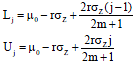 | (23) |
Let, cj denote the middle point of the j-th (j = 1, 2,…, 2m+1) interval, then we have:
| (24) |
Let, pij be the one-step transition probability from state i to state j when the progress is in control, then:
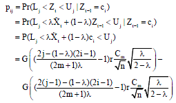 | (25) |
where, Φ(x) is the cumulative distribution of standard normal distribution.
Similarly, calculate the transition probability from state i to state j when the process is out of control p'ij, μ = μ0+aσ0, then:
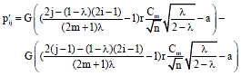 | (26) |
Define:
| (27) |
| (28) |
Then:
| (29) |
In a similar way ANOS1 can be written as:
| (30) |
COMPARISON OF FSS AND VSS EWMA MEDIAN CONTROL CHART
To compare the monitoring efficiency of control chart, we should make them have same ANOS when the process is under control. The ANOS rule was proposed by Costa (1994) and Reynolds (1996) and we can prove that ANOS = E(ni)ANSS, if n1, n2,… are independent and identically distributed. The ANSS here has the same meaning with ARL when the progress is nuder control (Costa, 1997).
Let N0 and N0 denote respectively the number of samples from beginning to signal when, μ = μ0 and μ = μ0+aσ. If μ = μ0, then N0 obey the geometric distribution of parameter q0,
Let:
| (31) |
Then the average sampling size is:
| (32) |
If μ = μ0+aσ, denote:
| (33) |
| (34) |
For VSS c-chart, select appropriate r' to make the formular established:
| (35) |
p01, p02 satisfy:
| (36) |
Then we can decide r' by Eq. 21.
Let λ take different values, select appropriate sampling size n1 and n1 to make the two charts have the same ANSS when μ = μ0. Then calculate the ANSS of the two control charts when μ = μ0+aσ0, the smaller the ANSS is, the higher the efficiency of the control chart will be.
For VSS c-chart, when μ = μ0, n = 5, r = 3, n1 = 3, n2 = 7, we have p02 = p01 = 0.4985 from Eq. 21. From Eq. 17, we get ![]() = 5, then we decide r' according to n.
= 5, then we decide r' according to n.
From G(c') = P ![]() = IΦ(c’) = (0.4985/2+0.5) = 0.74925. We get Φ(c') = 0.6401, c' = 0.3587. From r' cm/
= IΦ(c’) = (0.4985/2+0.5) = 0.74925. We get Φ(c') = 0.6401, c' = 0.3587. From r' cm/![]() = 0.3587, we get r' = 0.6699.
= 0.3587, we get r' = 0.6699.
In a similar way, we can calculate the average sampling size , then we can know ANSS.
COMPARISON OF MEAN AND MEDIAN CONTROL CHART
Then,we compare the ANSS of VSS mean and VSS median control chart. As well,select appropriate sampling size n1 and n2 to make the two charts have the same ANSS when μ = μ0. For n can only be integer here, so, we can only make both approximately equal.
CONCLUSION
From Table 1, we know that no matter what value the λ is, the ANSS of VSS EWMA control chart is smaller than that of FSS EWMA control chart when a is lager than 0.75. However, when a is lager than 0.75, the efficiency advantage is not so large.
From Table 2, we know that no matter what value the λ and a is, the ANSS of VSS median EWMA control chart is smaller than that of VSS EWMA mean control chart. Moreover, the advantage is much more obvious when the progress has a smaller offset. Just as we imagined, when the sampling result is good enough, we reduce the next sampling sample size, the other way around, we increase the sample size to discover the offset faster. So, the VSS control chart is more suitable than FSS control chart to apply to progress in practice. Besides, conventional control charts are monitoring the mean or variance, this study monitor the median and it has a more efficient result which is significant to the actual production.
| Table 1: | ANNS of FSS and VSS EWMA control charts |
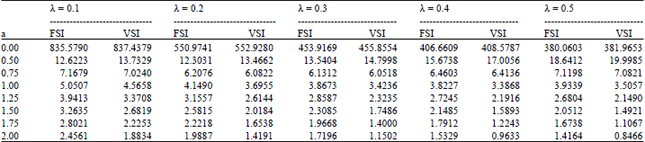 | |
| Table 2: | ANSS of VSS mean and VSS median control chart |
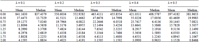 | |
ACKNOWLEDGMENT
This study is supported by the Science and Technology Research and Development Plan in China No. 201101B025.
REFERENCES
- Baxley, Jr. R.V., 1995. An application of variable sampling interval control charts. J. Qual. Technol., 27: 275-282.
Direct Link - Chang, S.Y. and D.S. Bai, 2001. Control charts for positively-skewed populations with weighted standard deviations. Qual. Reliabil. Eng. Int., 17: 397-406.
CrossRefDirect Link - Chou, C.Y., C.H. Chen and H.R. Liu, 2006. Economic design of EWMA charts with variable sampling intervals. Qual. Quant., 40: 879-896.
CrossRefDirect Link - Prabhu, S.S., D.C. Montgomery and G.C. Runger, 1994. A combined adaptive sample size and sampling interval X control scheme. J. Qual. Technol., 26: 164-176.
Direct Link - Reynolds, Jr. M.R. and J.C. Arnold, 2001. EWMA control charts with variable sample sizes and variable sampling intervals. IIE Trans., 33: 511-530.
CrossRefDirect Link - Reynolds, Jr. M.R., 1996. Variable-sampling-interval control charts with sampling at fixed times. IIE Trans., 28: 497-510.
CrossRefDirect Link - Roberts, S.W., 1959. Control chart tests based on geometric moving averages. Technometrics, 1: 239-250.
CrossRef - Saccucci, M.S. and J.M. Lucas, 1990. Average run lengths for exponentially weighted moving average control schemes using the Markov chain approach. J. Qual. Technol., 22: 154-162.
Direct Link