
Haiyan Xu
School of Informatics, Linyi University, Linyi, 276000, China
Information Technology Journal
Year: 2012 | Volume: 11 | Issue: 11 | Page No.: 1626-1631


ABSTRACT
This study proposed a novel framework for ear recognition based on Gabor wavelets and Support Vector Machine (SVM). The framework has three steps. In the first step, the ear is detected from an image of the face. In the second step, Gabor wavelets are used to extract ear feature. The Gabor wavelets, whose kernels are similar to the 2D receptive field profiles of the mammalian cortical simple cells, exhibit desirable characteristics of spatial locality and orientation selectivity. In the third step, when the Gabor features were obtained, classifications were done by SVM. Experiment results showed that the proposed framework is effective and accurate.
PDF Abstract XML References Citation
Received: March 20, 2012;
Accepted: June 18, 2012;
Published: August 28, 2012
How to cite this article
Haiyan Xu, 2012. The Research of Ear Recognition Based on Gabor Wavelets and Support Vector Machine Classification. Information Technology Journal, 11: 1626-1631.
DOI: 10.3923/itj.2012.1626.1631
URL: https://scialert.net/abstract/?doi=itj.2012.1626.1631
DOI: 10.3923/itj.2012.1626.1631
URL: https://scialert.net/abstract/?doi=itj.2012.1626.1631
INTRODUCTION
Recent years, biometrics has a rapid development because of its broad applications ranged from identification to security. Fingerprints, irises, faces, gait and speech are always used as popular biometrics. Because of ideal properties, such as university, uniqueness, permanence and so on, ear becomes a new class of biometrics (Chang et al., 2003; Iannarelli, 1989; Jain et al., 1999). Researchers have presented that each individual has different ears, from shape to appearance and the ear will never change during one’s lifetime (Iannarelli, 1989). Comparing to other population biometrics, ear has not received much attention though it has advantages over other biometrics.
Iannarelli (1989) used ear shape as features to distinguish between people. He made a foundation of ear recognition. Victor et al. (2002) and Chang et al. (2003) proposed a PCA (Principle Component Analysis) method to recognize ears. Hurley et al. (2002) used a new approach of FFT (Force Field Transformation) to extract features of ear. Yuizono et al. (2002) proposed a new framework of recognition by using genetic local search. Chen and Bhanu (2007) used a novel local surface shape descriptor and ICP (Iterative closest Point) procedure in 3D ear recognition system. Yuan and Mu (2012) presented a 2D ear recognition methodology by using local information fusion and part-covered ears can be recognized. Localized orientation information is used by Kumar and Wu (2011) as a new feature extraction approach to identify ears.
In this study, a novel framework for ear recognition based on Gabor wavelets and support vector machine was proposed, the framework contains three steps: ear detection, ear feature extraction and era recognition.
EAR DETECTION
Before ear feature extraction and ear recognition, ear should be detected from a person’s side face. In order to extract an image contains only the ear, there are three steps. First, skin-tone detection is used to detect a person’s side face containing the ear. Second, contour extraction is applied to the skin region and removes short and isolate edges. Third, the ear is located by segmentation from other skin region. Then, the detected ear is normalized to 45x80. Figure 1 depicts the ear detection from a face. And the procedure of ear recognition is shown as Fig. 2.
GABOR FEATURE EXTRACTION
Gabor wavelets: The Gabor wavelets are similar to human vision system, so they have been widely used in recognition applications, such as face recognition, fingerprint recognition, character recognition, etc. This feature based method aims to find the important local features and represent the corresponding information in an efficient way. Gabor wavelet was first proposed by Gabor (1946) for 1D signal decomposition and was extended to 2D domain by Granlund (1978) for analyzing 2D image. Shen and Bai (2008) have also applied 3D Gabor wavelets to evaluate 3D image registration algorithms. In the space domain, the 2D Gabor filter can be considered as a Gaussian kernel modulated by a sinusoidal plane wave. The Gabor wavelets can be defined as follows:
| (1) |
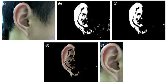 | |
| Fig. 1(a-e): | Ear detection, (a) Original image of right face containing right ear, (b) Image with contour extraction and filling, (c) Image after smoothing, (d) Result of segmentation and (e) Normalized ear image |
 | |
| Fig. 2: | The stages of ear recognition |
The parameter u defines the orientation of the Gabor kernels and the parameter v defines the scale of the Gabor kernels, z = (x, y), ||.|| denotes the norm operator and the wave vector ku,v is defined as follows:
| (2) |
where, kv = kmax/fv and φu = uπ/U, kmax is the maximum frequency and f is the spacing factor between kernels in the frequency domain (Laddes et al., 1993).
From only one Gabor filter, with different scale and orientation via the wave vector ku,v, all the Gabor kernels in Eq. 1 can be generated, so they are all self-similar.
 | |
| Fig. 3: | Gabor kernels (real part with five scales and eight orientations) |
Each kernel is a product of a Gaussian envelope and a complex plane wave, while the first term in the square brackets in Eq. 1 determines the oscillatory part of the kernel and the second term compensates for the DC value. The parameter σ determines the ratio of the Gaussian window width to wavelength (Li et al., 2011).
vε{0, 1, 2, …, V-1} is scale label, in most cases the use of Gabor wavelets of five different scales, so V = 5. uε{0, 1, 2, …, U-1} is orientation label and the Gabor wavelets are usually used eight orientations, so U = 8. With the following parameters: ![]() the kernels exhibit desirable characteristics of spatial frequency, spatial locality and orientation selectivity (Liu and Wechsler, 2002). The Gabor Kernels are shown in Fig. 3.
the kernels exhibit desirable characteristics of spatial frequency, spatial locality and orientation selectivity (Liu and Wechsler, 2002). The Gabor Kernels are shown in Fig. 3.
Representation of Gabor feature: The Gabor wavelet representation of an image can be obtained by convolving the image with a family of Gabor kernels as defined by Eq. 1. Let I (x, y) be the gray level distribution of an image and define the convolution output of image I and a Gabor kernel Ψu,v as follows:
| (3) |
where, z = (x, y) and * denotes the convolution operator. G (z) is the convolution result. As described V = 5, U = 8, 40 Gabor filters are made, the set S = {Gu,v (k, z):uε{0, …, 3}, vε{0, …, 7}} forms the Gabor wavelet representation of the image I (z). Where Gu,v (k, z) = |I (z)*G (k, z), all the Gabor features can be described as G (I) = G = (G0,0G0,1…G4,7). Taking an image of size 128x128 for example, the Gabor feature vector will be 128x128x5x8 = 655360 dimensions which is incredibly large. Due to the large number of convolution operations, the computation and memory cost of feature extraction is also necessarily high. So each Gu,v (k, z) is downsampled by a factor r. For a 128x128 image, the vector dimension is 10240 when the downsampling factor r = 64.
CLASSIFICATION BASED ON SUPPORT VECTOR MACHINE
Overview of support vector machine: The foundations of Support Vector Machines (SVM) have been developed by Vapnik (Boser et al., 1992). SVM is based on results from statistical learning theory. The basic idea of SVM is to map the input space to a higher dimensional feature space and to classify the transformed feature by a hyper-plane (Wu and Zhao, 2006; Pugazhenthi and Rajagopalan, 2007; Shao et al., 2008; Hung and Liao, 2008; Liejun et al., 2008; Lei and Zhou, 2012). SVM has become one of the most useful approaches in machine learning field due to its good performance of resolving classification problems (Sani et al., 2010; Yao et al., 2012). Consider the problem of separating the set of labeled training vectors belonging to two separate classes:
with a hyper-plane:
| (4) |
When the distance between the closest vector to the hyper-plane is maximal and it is separated without error, it is said the hyper-plane separates the set of vectors optimally and this hyper-plane is called Optimal Separating Hyper-plane (OSH). A separating hyper-plane in canonical form must satisfy the following constraints:
| (5) |
learning systems typically try to find a decision function of the form:
| (6) |
The coefficients a*i and b* in Eq. 6 are the solutions of a quadratic programming problem.
For non-linearly separable data, a non-linear mapping function Φ that embeds input vectors into feature space, kernels have the form:
| (7) |
SVM algorithms separate the training data in feature space by a hyper-plane defined by the type of kernel function used. The kernel functions used are:
| • | Linear kernel: k (x, xi) = (x, xi) |
| • | Radial Basis Function (RBF): K (x, xi) = exp (-||x-xi||2/2σ2) |
| • | Polynomial: K (x, xi) = [⟨x, xi⟩+1]d |
| • | Sigmoid: K (x, xi) = tanh (α⟨x, xi⟩+c) |
The SVM methodology learns nonlinear functions of the form:
| (8) |
Multi-class classifications: A multi-class classification can be obtained by composition of two-class SVMs. There are two main strategies to deal with multi-class classification. One is the one-against-all strategy to classify between each class and all the remaining, it needs to construct k SVMs where k is the number of lasses, in each SVM, all data must be included in training. Another is the one-against-one strategy to classify between each pair, only two classes data are used in each SVM, as a tradeoff, k (k-1)/2 classifiers have to be constructed (Mohammadi and Gharehpetian, 2008). Because of the one-against-all strategy often leads to ambiguous classification (Pontil and Verri, 1998), so one-against-one strategy was adopted in our system and the RBF kernel is used.
A bottom-up binary tree is constructed for classification. Take an eight-class data set for example, the decision tree is shown in Fig. 4. We encode each class with numbers from 1 to 8 and the numbers are arbitrary without any means of ordering. One class number will be chosen representing the “winner” of the current two classes after comparison between each pair and the selected classes from the lowest level of the binary tree will come to the upper level for another round of tests. Finally, the unique class will appear on the top of the tree.
Suppose the number of classes as k, the SVMs will learn k (k-1)/2 discrimination functions in the training stage and each binary tree has k-1 times comparisons.
 | |
| Fig. 4: | The binary tree with 8 classes |
According to the methodology proposed by Guo et al. (2000), if k does not equal to the power of 2, we can decompose k as k = 2n1+2n2+…+2nl, n1≥n2≥…≥nl. Thus every natural number can be decomposed to power of 2, when is k odd, nl = 0; otherwise, when k is even, nl≥0. Although the decomposition is not unique, the binary tree always has times comparisons.
EXPERIMENTS
The toolbox libsvm (Chang and Lin, 2001) is used as the underlying SVM classifier. In our experiments, we choose 40 volunteers as our subjects. We take 10 images with right face containing ear for each subject. These images are taken under different view conditions and different illumination conditions. Besides, the distance between camera and subject is considered. Figure 5 shows images of ears with one subject.
The normalized ear images with a resolution of 45x80, 40 Gabor filters are used to extract features, the Gabor feature vector of each ear image will be 45x80x5x8 = 14400 dimensions. Downsampling Gabor feature vector by factor r = 64, the vector dimension is reduced to 225. Forty subjects take part in the experiment, that means 40 classes, so the number of classes k = 40, each class contains 10 images, thus, we have 400 ear images in total. Decomposing 40 = 32+8, two binary tree are constructed, one with 32 leaves and the other with 8 leaves. Then compare the two outputs to determine the true class in another binary tree with only two leaves. The times of comparisons for one query are 39. Five ear images are selected at random from each subject as training set and the other 5 ear images as test set, both training set and test set have 5x40 = 200 images. The experiments are repeated for 5 times.
In order to evaluate the performance of the proposed method in ear recognition, some widely-used methods are compared with: such as Principal Components Analysis (PCA) (Victor et al., 2002; Chang et al., 2003), Linear Discriminant Analysis (LDA) (Zhang and Jia, 2007), Fisher Discriminant Analysis (FDA) (Liu et al., 2006), rotation invariant descriptor (Fabate et al., 2006), Local Binary Pattern (LBP) (Ahonen et al., 2006). Those methods are also tested on our ear dataset.
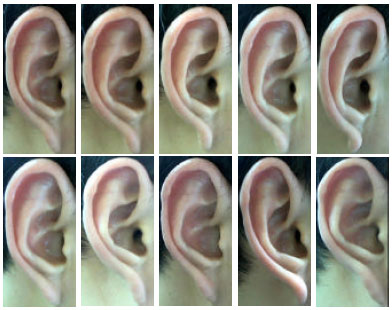 | |
| Fig. 5: | Ears of one subject |
| Table 1: | Experimental results of ear recognition via different methods |
 | |
From Table 1, we can observe that the proposed framework performs well in ear recognition.
CONCLUSION AND FUTURE WORK
In this study, a novel approach of ear recognition are presented, ears are detected from person’s side face, then Gabor wavelets are used for feature extraction and multi-class SVM classification with binary tree strategy is performed for ear recognition. The experimental results showed the proposed framework perform better than methods in some literatures. The ear biometrics has the potential to be used in application to identify or recognize humans by their ears. Also, the ear biometrics can be combined with other biometrics as security application. In the further work, the author will focus on the recognition with part-covered ear and the dimension reduction of Gabor feature.
ACKNOWLEDGMENTS
The author would like to thank all the volunteers for screening their ears to form the ear dataset which is used in this study.
REFERENCES
- Ahonen, T., A. Hadid and M. Pietikainen, 2006. Face description with local binary patterns: Application to face recognition. IEEE Trans. Pattern Anal. Mach. Intell., 28: 2037-2041.
CrossRefDirect Link - Boser, B.E., I.M. Guyon and V.N. Vapnik, 1992. A training algorithm for optimal margin classifiers. Proceedings of the 5th Annual Workshop on Computational Learning Theory, July 27-29, 1992, Pittsburgh, Pennsylvania, USA., pp: 144-152.
CrossRef - Chang, K., K.W. Bowyer, S. Sarkar and B. Victor, 2003. Comparison and combination of ear and face images in appearance-based biometrics. IEEE. Trans. Patt. Anal. Mach. Intel., 25: 1160-1165.
CrossRef - Chen, H. and B. Bhanu, 2007. Human ear recognition in 3D. IEEE Trans. Pattern Anal. Machine Intell., 29: 718-737.
CrossRefDirect Link - Granlund, G.H., 1978. In search of a general picture processing operator. Comput. Graphics Image Process., 8: 155-173.
CrossRef - Hurley, D.J., M.S. Nixon and J.N. Carter, 2002. Force field energy functional for image feature extraction. Image Vision Comput., 20: 311-317.
CrossRef - Hung, Y.H. and Y.S. Liao, 2008. Applying PCA and fixed size LS-SVM method for large scale classification problems. Inform. Technol. J., 7: 890-896.
CrossRefDirect Link - Kumar, A. and C. Wu, 2012. Automated human identification using ear imaging. Pattern Recog., 45: 956-968.
CrossRefDirect Link - Laddes, M., J.C. Vorbruggen, J. Buchman, J. Lange, C. van der Malsburg, R.P. Wurtz and W. Konen, 1993. Distortion invariant object recognition in the dynamic link architecture. IEEE Trans. Comput., 42: 300-311.
CrossRefDirect Link - Lei, X. and P. Zhou, 2012. An intrusion detection model based on GS-SVM Classifier. Inform. Technol. J., 11: 794-798.
CrossRefDirect Link - Li, W., Y. Lin, H. Li, Y. Wang and W. Wu, 2011. Multi-channel gabor face recognition based on area selection. Inform. Technol. J., 10: 2126-2132.
CrossRefDirect Link - Liu, C. and H. Wechsler, 2002. Gabor feature based classification using the enhanced fisher linear discriminant model for face recognition. Image Proc. IEEE Trans., 11: 467-476.
CrossRefDirect Link - Pontil, M. and A. Verri, 1998. Support vector machines for 3D object recognition. IEEE Trans. Pattern Anal. Mach. Intell., 20: 637-646.
CrossRefDirect Link - Mohammadi, M. and G.B. Gharehpetian, 2008. Power system on-line static security assessment by using multi-class support vector machines. J. Applied Sci., 8: 2226-2233.
CrossRefDirect Link - Pugazhenthi, D. and S.P. Rajagopalan, 2007. Machine learning technique approaches in drug discovery, design and development. Inform. Technol. J., 6: 718-724.
CrossRefDirect Link - Shen, L. and L. Bai, 2008. 3D Gabor wavelets for evaluating SPM normalization algorithm. Med. Image Anal., 12: 375-383.
CrossRef - Shao, F., H. Duan, G. He and X. Zhang, 2008. A unified model for privacy-preserving support vector machines on horizontally and vertically partitioned data. Inform. Technol. J., 7: 850-858.
CrossRefDirect Link - Sani, M.M., K.A. Ishak and S.A. Samad, 2010. Classification using adaptive multiscale retinex and support vector machine for face recognition system. J. Applied Sci., 10: 506-511.
CrossRefDirect Link - Victor, B., K. Bowyer and S. Sarkar, 2002. An evaluation of face and ear biometrics. Proc. Int. Conf. Pattern Recog., 1: 429-432.
CrossRef - Liejun, W., J. Zhenhong and L. Zhaogan, 2008. Multi-resolution signal decomposition and approximation based on SVMS. Inform. Technol. J., 7: 320-325.
CrossRefDirect Link - Wu, F. and Y. Zhao, 2006. Least squares support vector machine on morlet wavelet kernel function and its application to nonlinear system identification. Inform. Technol. J., 5: 439-444.
CrossRefDirect Link - Yuan, L. and Z.C. Mu, 2012. Ear recognition based on local information fusion. Pattern Recog. Lett., 33: 182-190.
CrossRef - Yao, Y., L. Feng, B. Jin and F. Chen, 2012. An incremental learning approach with support vector machine for network data stream classification problem. Inform. Technol. J., 11: 200-208.
CrossRefDirect Link - Zhang, X. and Y. Jia, 2007. Symmetrical null space LDA for face and ear recognition. Neuro-Computing, 70: 842-848.
CrossRef