
Geng Yuefeng
College of Electrical and Information Engineering, Xuchang University, Xuchang 461000, China
Information Technology Journal
Year: 2013 | Volume: 12 | Issue: 4 | Page No.: 704-711


ABSTRACT
The spatial redundant robot model was established, its inverse kinematics solution was derived and chaotic motion in zero space self-motion was analyzed; the potential function was constructed by artificial potential field method for the chaotic motion in the zero space self-motion. Simulation results showed that chaotic motion in zero space self-motion of the spatial redundant robot changed into regular motion after joining the potential function in the inverse kinematics solutions of the spatial redundant robot, therefore, the artificial potential field method as chaotic motion control of the spatial redundant robot algorithm was effective.
PDF Abstract XML References Citation
Received: September 07, 2012;
Accepted: November 24, 2012;
Published: January 22, 2013
How to cite this article
Geng Yuefeng, 2013. Chaos Control Algorithm for Redundant Robotic Obstacle Avoidance. Information Technology Journal, 12: 704-711.
DOI: 10.3923/itj.2013.704.711
URL: https://scialert.net/abstract/?doi=itj.2013.704.711
DOI: 10.3923/itj.2013.704.711
URL: https://scialert.net/abstract/?doi=itj.2013.704.711
INTRODUCTIONS
Redundant robot is the number of degrees of freedom more than the dimensions of the task space (Lu, 2007). Such robots can realize the motion law of the end-effector and can improve the dexterity, obstacle avoidance capability and dynamic performance to avoid joint overrun of the robot simultaneously by using of the self-motion of the zero space (Xinfeng, 2012). Therefore, the redundant robot has become a hot research in the field of mechanical engineering and automatic control for its great potential advantage applications in the manufacturing industry. The self-motion of redundant robot can lead to the chaotic motion generated (Yin and Ge, 2011), the chaotic motion will bring great difficulties to the robot control. Therefore, to make use of the advantages while avoiding chaotic motion in the redundant robot control process.
Controlling the chaotic motion means that the additional performance optimization is added in redundant robot zero space. In actual industrial field, there will be many obstacles exist due to the limitations of the workspace; the redundant robot should avoid collision with the obstacles. The main avoiding robot obstacle methods are geometric method (Nektarios and Aspragathos, 2010), genetic algorithms (Li et al., 2012) and artificial potential field method (Klein, 1984), geometric method and genetic algorithm are global planning, the search time is long, the hardware requirements is high and the real-time control is difficult. The artificial potential field method can not guarantee that the conclusion is the global optimum, but the obstacle avoidance potential function is easy to construct and the computing time is short, the real-time control is facilitated to realize. Research on obstacle avoidance planning has made many achievements based on artificial potential field since the artificial potential field method is proposed for the first time by Khatib (1986) and Ye and Wang (2012).
An obstacle avoidance potential function to avoid the collision with multiple obstacles in the workspace is constructed based on the study of Mohri et al. (1995) in this study, the obstacle avoidance potential function is applied to solve the inverse kinematics problem of the redundant robot, simulation results show that the chaotic motion become a fixed periodic orbits motion that inverse kinematics solution of redundant robot is optimized by the obstacle avoidance potential function.
THE CHAOTIC MOTION ANALYSIS IN THE SPATIAL REDUNDANT ROBOT SELF-MOTION
The spatial redundant robotic manipulator’s model: Because of the spatial robotic body is not fixed, reaction and torque to the robotic body will be generated by motion of the robotic manipulator and caused position and posture of the robotic body change, the position and posture changes of the robotic body in turn affect positioning of the robotic manipulator, thus affecting the end-effector’s operational planning, so the free-floating spatial redundant robotic manipulator’s kinetic characteristics are very different from the fixed base robotic manipulator’s (Vakakis and Burdick, 1990). Establish inertial coordinate system ΣI which fixed on center of mass of system, joint coordinate system Σi which fixed on the ith joint, D-H parameters of joint coordinate system according to D-H parameters method (Denavit and Hartenberg, 1995), body coordinate system Σ0 which fixed on center of mass of the body, the position and posture which body coordinate system relative to inertial coordinate system are expressed by the position vector r0 and Z-Y-X Euler angles α, β, γ (Fig. 1):
| ΣI | = | Inertial coordinate system that fixed on the system centroid |
| ΣI | = | Joint coordinate system that fixed on the ith joint of the robotic manipulator |
| m0,i0 | = | The mass and inertia moment of the basic body |
| mi,Ii | = | The mass and inertia moment of the ith link |
| r0 | = | The position vector from the origin of the inertial coordinate system to the origin of the basic body coordinate system |
| rci | = | The position vector from the origin of the inertial coordinate system to the ith link centroidcoordinate system |
| pi | = | The position vector expressed in the ith link coordinate system from the origin of the ith link coordinate system to the centroid |
| ii-1l | = | The position vector expressed in the (i-1)th link coordinate system from the origin of the (i-1)th link coordinate system to the origin of the ith link coordinate system |
| = | The angular velocity vector of the robotic manipulator ith joint | |
| ωi | = | The angular velocity of the robotic manipulator’s ith joint expressed in the joint coordinate system that fixed on the ith joint of the robotic manipulator |
| vi | = | The line velocity of the robotic manipulator ith joint expressed in the joint coordinate system that fixed on the ith joint of the robotic manipulator |
| ωic | = | The angular velocity of the robotic manipulator’s ith joint centroid expressed in the joint coordinate system that fixed on the ith joint of the robotic manipulator |
| vic | = | The line velocity of the robotic manipulator’s ith joint centroid expressed in the joint coordinate system that fixed on the ith joint of the robotic manipulator |
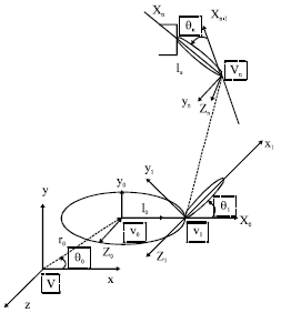 | |
| Fig. 1: | The spatial redundant robotic manipulator model of n joints |
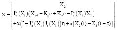
Inverse kinematics of the spatial redundant robot: Kinematics manipulability W of the spatial redundant robotic manipulator is select as optimal objective function of avoiding singular, PD controller is designed to make the end-effector track the closed curve of the robotic work space repeatedly, joint acceleration expression can be obtained based on the pseudo-inverse of Jacobian matrix:
| (1) |
Therein, ![]() is the gradient of manipulability function, Kv = kv*I, Kp = kp*I, kv, kp are the magnification times of the displacement error and velocity error, respectively, I is unit matrix,
is the gradient of manipulability function, Kv = kv*I, Kp = kp*I, kv, kp are the magnification times of the displacement error and velocity error, respectively, I is unit matrix, ![]() is the desired acceleration of the end-effector, ep = pd-Xed,
is the desired acceleration of the end-effector, ep = pd-Xed, ![]() are the position deviation and velocity deviation of the end-effector, respectively. Scalar magnification coefficient a = 1.
are the position deviation and velocity deviation of the end-effector, respectively. Scalar magnification coefficient a = 1.
In order to facilitate research, the state variables defined as follows:
| (2) |
Therein, X1 = Q = [Q0, Q1, Q2, L, Qn]T, X2 = Q = [Q0, Q1, Q2,..., Qn]T.
The original system equation can be expressed as:
| (3) |
The chaotic motion analysis: The 3 joints redundant spatial robotic manipulator operated plane motion which is taken as an example and computer numerical simulation is made in this study. Simulation requires the end-effector moving by desired trajectory.
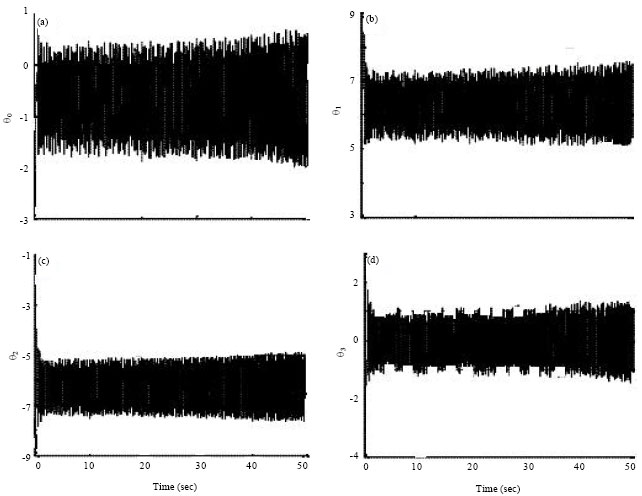 | |
| Fig. 2(a-d): | The time course of qi |
System parameters are as follows: the body mass is m0 = 1 kg, each link mass are m1 = m2 = m3 = 1 kg, i0 1 kg m2 the body rotary inertia is i0 = 200 kg m2, each link rotary inertia are i1 = 0.3 kg m2, i2 = 0.2 k g2, i3 = 0.1 kg m2, the length of links are l1 = l2 = l3 = 1 m, the distance from the body center of mass to the first joint is l0 = 1 m, position vector of the body center of mass in inertial coordinate system is rI = (0,0.2), the desired trajectory, the desired velocity and the desired acceleration of the end-effector are, respectively:
 | (4) |
By simulation we can see that different initial shape of the free-floating spatial redundant robotic manipulator and coefficient kv, kp which make system closed-loop stability can lead to chaotic motion of the spatial redundant robotic system. Limited space, here only given a set of values simulation results:
| (5) |
Initial shape:
| (6) |
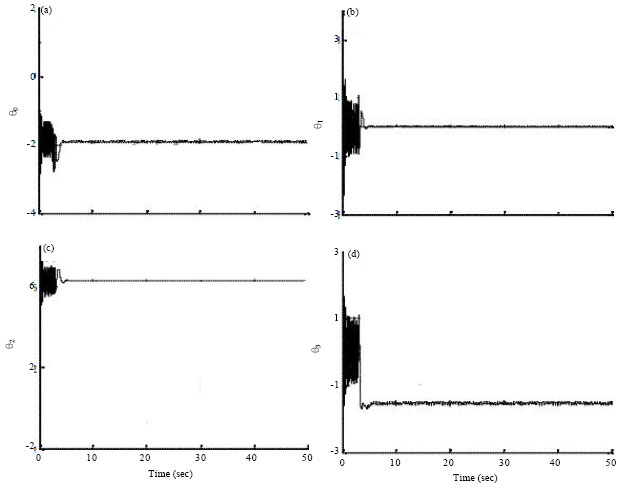
To further observe the system’s self-motion state, the time course of the joint figure, phase figure and Poincare section are drawn and as shown in Fig. 2-4.
From the time course can be seen that the base angle and joint angle changes over time showed the characteristics of chaotic motion. During the experiment, modify the initial value of the robotic system, the time course of the robotic system has greatly changed which indicates the initial sensitivity of the robotic system.
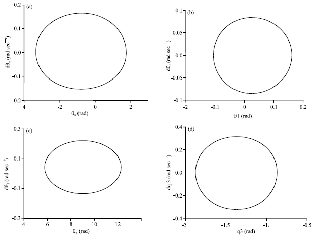
From Fig. 3 can be seen that the phase trajectory is randomly distributed, neither overlap nor intersect, repeated folding in a certain area. There is chaotic motion in redundant spatial robotic system at initial judgments.
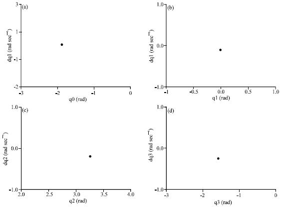
From Fig. 4 can be seen that Poincare section composed by an infinite number of discrete points. The self-motion of robotic system has characteristics of chaotic motion for the nature of the Poincare section.
A large number of numerical simulations are exercised by chaos analysis method such as direct observation, time-course method, phase figure and Poincare section method.
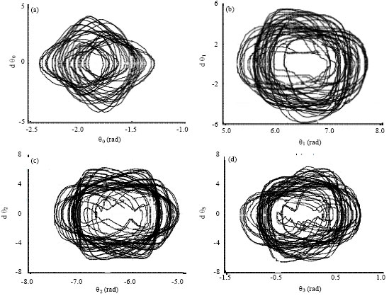 | |
| Fig. 3(a-d): | Phase figure of qi |
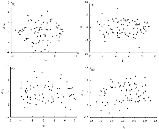 | |
| Fig. 4(a-d): | Poincare section of qi |
The results show that: the free-floating redundant spatial robotic manipulator’s self-motion is chaotic when solving the robotic manipulator’s inverse kinematics based on pseudo-inverse Jacobian matrix, designing PD controller to make the end-effector track the closed curve of the robotic work space repeatedly.
INVERSE KINEMATICS SOLUTIONS BASED ON THE OBSTACLE AVOIDANCE POTENTIAL FUNCTION
The artificial potential field method: Assumed the robotic links are straight and each of the obstacles in the workspace can be included in a sphere, as shown in Fig. 5.
Obstacle avoidance potential function can be constructed using the geometric relationship between the robot and obstacle, the distance between link jth and obstacle ith is as follow:
| (7) |
where, k is the number of obstacles; n is the number of joints; Oi is the position vector of the obstacle ith; Pj is the position vector of the joint jth.
The distance between joint jth and obstacle ith is:
| (8) |
Obstacle avoidance potential function is:
| (9) |
where, when {d1ij-ri-si}< 0 and Dij locate between Pj and Pj+1, F1ij (q) = (d1ij-ri-si)2, otherwise F1ij (q) = 0; when (d2ij-ri-si)<0, (d2ij-ri-si)2, otherwise F1ij (q) = 0; W1 and W2 are positive constant; ri is the radius of the sphere, si is safety factor, Dij is the foot of a perpendicular line from the center of the obstacle ith to the link jth.
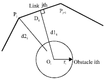 | |
| Fig. 5: | The relative position of the robot with the obstacle |
Assumed the robot task is tracking a plane round, the desired trajectory of the end-effector is shown in formula (4). W1 and W2 take as 2, si take as 0.1, the obstacle avoidance potential function is:
| (10) |
Inverse kinematics solutions based on the obstacle avoidance potential function: The redundant robotic acceleration inverse solution based on the Jacobian matrix pseudo-inverse under avoiding obstacles is expressed as:
| (11) |
where, η = ∇h (q)∈R3x1 is the gradient of the obstacle avoidance potential function, substitute the formula (2) and (10) into (11) and transformed the formula (11) into the first-order differential equations, such as:
| (12) |
CHAOS MOTION CONTROL RESULTS AND ANALYSIS
Chaos control algorithm procedure is as follows:
The first step, selected the obstacle avoidance potential function; the second step, optimized the redundant robotic manipulator inverse kinematics taking use of the selected obstacle avoidance potential function as a secondary task; the third step, simulated kinematics according to the optimization results by added the perturbation signal.
After adding perturbation control signal N(t) = μ [y(t)-(t-t)], The formula (12) becomes:
 | (13) |
The relation between the largest Lyapunov exponent λmax of the system and the delayed feedback coefficient K is shown in Fig. 6. when 1.3<μ2.3 and λmax<0, the spatial redundant robot system changed into regular motion state.
The desired period of the spatial redundant robot is T = 2π/ω = 1 sec, take τ = T = 1 sec, a group disturbance weighting value that can control the chaotic motion is selected, the other parameters are the same as before.
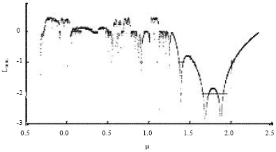 | |
| Fig. 6: | The relation between λmax and K |
 | |
| Fig. 7(a-d): | The time course of qi after mixed the delayed feedback control |
In order to obtain information of the original system fully, the delayed feedback control is mixed for further study after 5 sec. Figure 7-9 are the time course figure of qi, the phase figure of qi, the Poincare section figure of qi, these figures confirmed that the system has been converted to the periodic motion.
 | |
| Fig. 8(a-d): | Phase figure of qi after mixed the delayed feedback control |
 | |
| Fig. 9(a-d): | Poincare section of qi after mixed the delayed feedback control |
CONCLUSIONS
The self-motion of the spatial redundant robot system is studied in simulation; the results showed that the self-motion state of the redundancy spatial robotic is chaotic. the delay time τ is used for the desired period and the corresponding figure between the feedback weighting coefficient k and its motion state is drawn according to the characteristics of chaotic motion. The chaotic motion in self-motion of the spatial redundant robot is converted to the periodic motion rapidly selecting the appropriate control parameters.
ACKNOWLEDGMENT
This study is financially supported by National Natural Science Foundation of China (51275479).
REFERENCES
- Xinfeng, G.E. and Z. Dongbiao, 2012. Parameterized self-motion manifold of 7-DOF automatic fiber placement robotic manipulator. J. Mech. Eng., 48: 27-31.
CrossRefDirect Link - Yin, Z.F. and X.F. Ge, 2011. Chaotic self-motion of a spatial redundant robotic manipulator. Res. J. Applied Sci. Eng. Technol., 3: 993-999.
Direct Link - Nektarios, A. and N.A. Aspragathos, 2010. Optimal location of a general position and orientation end-effector's path relative to manipulator's base, considering velocity performance. Rob. Comput. Integr. Manuf., 26: 162-173.
CrossRef - Li, Q., L.J. Wang, B. Chen, Z. Zhou and Y.X. Yin, 2012. An improved artificial potential field method with parameters optimization based on genetic algorithms. J. Univ. Sci. Technol., 34: 202-206.
Direct Link - Khatib, O., 1986. Real-time obstacle avoidance for manipulators and mobile robots. Int. J. Robot. Res., 5: 90-98.
CrossRefDirect Link - Mohri, A., X.D. Yang and M. Yamamoto, 1995. Collision free trajectory planning for manipulator using potential function. Proceedings of the IEEE International Conference on Robot and Automation, Volume 3, May 21-27, 1995, Nagoya, Japan, pp: 3069-3074.
CrossRef - Vakakis, A.F. and J.W. Burdick, 1990. Chaotic motions in the dynamics of a hopping robot. Proceedings of the IEEE International Conference on Robotics and Automation, Volume 3, May 13-18, 1990, Cincinnati, OH., USA., pp: 1464-1469.
CrossRef - Denavit, J. and R.S. Hartenberg, 1955. A kinematic notation for lower-pair mechanisms based on matrices. Trans. ASME J. Applied Mech., 23: 215-221.
Direct Link